Verify Factory Energy Savings with a Measurement and Verification Plan

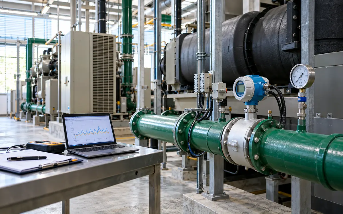
A lower bill leaves an engineering question open

A garment factory changes its pump controls. The next electricity bill falls by eight percent. The project team calls the change a success. Yet that month had fewer working days and cooler weather. Its product mix had changed too. The bill records what the factory bought. It does not, by itself, show how much the new controls saved.

Measurement and verification is usually called M&V. It asks a more precise question. Without the project, how much energy would the factory have used in this period? The answer needs a measured reference, a clear boundary and fair adjustments. It also needs evidence that the factory still delivered the required service.

EVO's public explanation of IPMVP makes this distinction clear. Savings represent energy use that did not occur. They must be calculated from measured use and suitable adjustments. This guide develops an original factory example. It also describes the records needed to check the calculation.

Define the claim before choosing the meter

Define the project in one sentence. State the energy source, service, and reporting period. For example: “Verify electricity saved by revised chilled-water controls, while room conditions meet approved limits.” That sentence prevents several different claims from being mixed together.

Energy savings use units such as kWh or gigajoules. Demand savings use kW or kVA over a defined interval. Cost savings use money under a stated tariff. Carbon reductions require a separate emissions method and factors. A project can produce one of these benefits without producing all four.

Choose a measurement boundary that includes the equipment affected by the change. A chiller-only meter can miss an increase in pump or tower power. A whole-factory meter can hide a small chiller saving beneath changes in production. Draw the boundary on the electrical and process diagrams. List each meter that crosses it.

Specify the service conditions too. These might include water flow, room conditions, steam pressure or accepted output. Less cooling may make the sewing floor too warm. Explain that service change in the result. The comparison should reflect the performance the project was intended to deliver.

Keep the wider investment decision in the factory's capital project review. The M&V record supplies energy evidence. The full financial review is still needed.

Agree a short plan while the old equipment still runs

Baseline evidence is easiest to collect before work begins. The work may remove an old motor or control sequence. It may change the schedule. Afterward, the former system may be impossible to measure directly. Agree the plan early enough to capture representative operation.

The plan should make another engineer able to reproduce the result. It needs more than a sentence promising to check future bills. The following structure is a practical starting point for a factory. It is not tied to one contract form.

The FEMP M&V planning resources provide useful examples of formal plan structure. Their contract requirements serve US federal projects. A textile factory can use the same planning logic. Apply the contract and operating rules that govern its own work.

Match the method to the decision

The four familiar IPMVP options describe different measurement approaches. They do not rank projects from poor to good. Choose based on the boundary and expected saving. Consider how operation varies and what evidence is already available.

The DOE explanation of M&V options describes these approaches. The practical question is which uncertainty matters for the proposed claim. Measuring lamp power very well will not resolve uncertain annual operating hours. Other loads may change each week. A whole-factory bill cannot then isolate one small machine.

A more complex model also needs more maintenance. Choose a method the factory can sustain after the consultant leaves. Record why the method was chosen. Include the cost of collecting and reviewing data.

Build a baseline that represents the old system

A baseline is a description of measured operation over a defined period. It may use fixed power and hours or a set of load bins. A model can also relate energy to key operating variables. It should reflect normal use as well as known operating limits.

Collect enough data to cover conditions that are likely to affect the result. A cooling project may need different weather conditions. A dyehouse project may need light and heavy production weeks. A short trial may cover only one easy style. It can be a weak reference for later orders.

Preserve the raw data before cleaning it. Mark outages, meter faults, trial runs and missing records with reasons. Keep high-energy weeks in the record. Treat one separately only when a valid reason is documented.

Use variables that describe demand on the system. Examples include production quantity, operating hours and weather. Be careful with a variable changed by the retrofit itself. A control project may reduce fan runtime. Adjusting both periods to the new runtime can then remove part of the benefit.

The DOE energy intensity guide explains the effects of production and weather. Both can change an energy comparison. For a project, apply that principle within the agreed boundary. Do not add variables simply because a spreadsheet can fit them.

Check the model beyond its fit statistic

A high coefficient of determination can coexist with a poor savings estimate. Check that the model makes physical sense. Look for patterns in its errors. Compare reporting conditions with those used to build it.

Plot prediction errors against time, production and weather. Errors may stay positive on the night shift. The model may be missing an operating mode. An abrupt change after a meter replacement may indicate a data problem. A model may predict negative use at low output. Review that fault before using it to claim savings.

If enough baseline data exists, keep a portion for a prediction check. Compare predicted and measured use on that portion. A model may follow noise in the fitting data. This check shows whether it also works on new observations.

Also test the reporting inputs. Suppose the baseline covers 40,000 to 80,000 pieces per week. Applying it at 140,000 pieces is an extrapolation. The result may need more evidence or a revised method. Label that limitation clearly instead of hiding it in an annual total.

The BPA M&V resources distinguish several methods. These include engineering calculations, end-use measurements, and energy models. That distinction helps reviewers ask whether the evidence supports the chosen method.

Work through an adjusted factory comparison

The following figures are hypothetical. They illustrate the arithmetic. They do not describe an actual mill or fitted research model. They are not promised savings. Assume the factory has reviewed and accepted the following baseline model. It covers one building:

Expected weekly electricity, kWh = 8,000 + 0.12 × accepted pieces + 30 × cooling degree-days.

The constant and coefficients belong only to this example. Cooling degree-days use one agreed base temperature and one weather source throughout. Use the model for the same building loads and operating range. The reporting data must fit that boundary.

For week one, the calculation is 8,000 + 0.12 × 60,000 + 30 × 40 = 16,400 kWh. Subtracting the measured 14,600 kWh gives an initial saving of 1,800 kWh.

Across four weeks, the adjusted comparison gives 8,100 kWh. The initial saving rate is 8,100 ÷ 70,100 × 100 = 11.6 percent, rounded. Use the adjusted baseline as the denominator. It estimates the old system's energy need under reporting conditions.

Suppose the previous four calendar weeks used 66,000 kWh. A simple before-and-after comparison would show only 4,000 kWh, or 6.1 percent. The difference arises because the two periods had different operating demands. Check the adjustment method and its evidence to judge which comparison is useful.

Keep unusual changes separate from routine adjustment

Routine adjustments address variables already represented in the agreed method. A normal change in output or weather belongs here when the model covers it. Other changes may alter the system itself and require a separate, nonroutine adjustment.

Assume a new ventilation fan was added to the example building after the retrofit. It is unrelated to the project. Its separately measured use was 600 kWh during the reporting period. That is already part of the 62,000 kWh building total.

Assume the approved comparison includes the new fan as a load for both systems. The old system would also have served it. Add 600 kWh to the adjusted baseline:

Final adjusted baseline = 70,100 + 600 = 70,700 kWh.

Verified estimate of avoided use = 70,700 − 62,000 = 8,700 kWh.

The resulting rate is 8,700 ÷ 70,700 × 100 = 12.3 percent. For this adjustment, record the installation date and measurement basis. Include the approval too. It cannot simply be a balancing amount added to reach a target.

A removed load works in the other direction. Production may move outside the boundary. Revise the comparison so the retrofit does not gain credit for that move. Keep an event register. Include new equipment, shift changes, major maintenance, changed space, and replaced meters.

State uncertainty in units that a decision maker can use

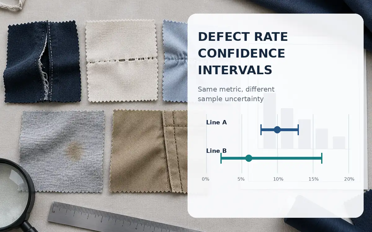
Savings are the difference between two quantities. Each may be much larger than the saving itself. Each quantity may have a small error. That error can be large relative to the saving. Meter accuracy is only one part of that uncertainty. Sampling, missing data, model prediction and adjustments also matter.

For this simple example, assume three independent standard uncertainties. Use 900 kWh for the adjusted model prediction. Use 300 kWh for reporting energy and 100 kWh for the extra-fan adjustment. These are assumed values, not estimates from the example's four rows.

Combined standard uncertainty = √(900² + 300² + 100²) = 954 kWh, rounded.

Assume a coverage factor of two. The expanded uncertainty is then about 1,908 kWh. This assumes a suitable distribution and degrees of freedom. Subject to those assumptions, report approximately 8,700 ± 1,908 kWh. That is about 22 percent of the central estimate. A real analyst must justify the uncertainties, correlations and coverage factor.

Do not attach a confidence percentage to an arbitrary high-and-low scenario. A sensitivity test and a statistical uncertainty interval answer different questions. Both can help, but each needs the right label.

ISO 50015:2014 gives general M&V principles for energy performance. ISO confirmed it in 2025. Its scope supports a planned, clear method. The public abstract gives no single uncertainty threshold for every project.

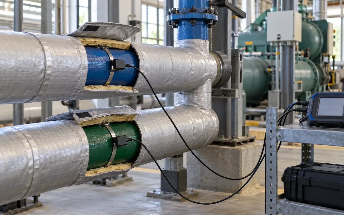
Convert energy into money after the energy result is clear

Use the agreed pricing basis to value the verified energy estimate. In the example, assume a constant comparison rate of USD 0.12 per kWh. The energy value is 8,700 × 0.12 = USD 1,044 for the four-week period.

Assume a verified billing-demand reduction is worth another USD 80. The gross cost benefit becomes USD 1,124. For the same period, assume added maintenance costs USD 60. M&V costs another USD 80. The resulting operating benefit is USD 984. Financing, tax, and other project costs are not yet included.

Those figures are hypothetical. Check the real tariff. Its demand charge may use a specific interval, a past maximum, or a minimum billed demand. An equipment peak reduction may leave the billed peak unchanged. Fixed service charges also remain unless the contract actually changes.

Prepare a bridge from energy change to price change. Finance can then see why the bill changed. The physical saving may have stayed similar. Use actual bill arithmetic for cash savings. Use the agreed common price basis for an engineering comparison.

Deal with interactions before adding project savings

Two projects can affect the same energy use. Better insulation may reduce boiler fuel. It may also leave less heat for a recovery system. New lighting may reduce electrical input while changing the building's cooling load. Adding independent estimates can double count the shared benefit.

Decide whether to measure the combined package or allocate the result among measures. Package verification is often easier when the measures interact strongly. Separate attribution may need more evidence. Agree an installation sequence, extra meters, or a calculation method before work starts.

The same rule applies to production changes. A new recipe may cut heating demand. A boiler project may change the fuel needed to meet that demand. Show each causal path clearly. Do not award the entire fuel reduction to both teams.

Use a versioned list of measures inside the boundary. A later project may need a baseline change. Decide whether to adjust or retire the old baseline. It may also be kept for a combined comparison. Otherwise, the factory can keep claiming the same saving against several overlapping references.

Test operation and then test persistence

Commissioning should confirm that the installed equipment performs its intended function. Observe the required flows, temperatures, pressures, control responses and product outcomes. An energy meter alone cannot prove that the right control sequence is running.

Then check whether the result lasts. A sensor can drift. A schedule can be changed. Operators may leave a manual override in place after a fault. Record these events and their effect on the claim. Do not treat every later increase as random variation.

The FEMP Version 5.0 guidelines cover planning, installation checks and performance-period verification. Link the energy evidence to the conditions in which it was measured. Equipment may be capable of saving energy. The report must show what savings were demonstrated during the period.

Choose review frequency from the consequence of drift and the pace of change. A stable lighting circuit may need fewer checks. A control system with daily overrides may need more. Match inspection effort to the remaining uncertainty and value at stake.

Make missing data visible

A blank interval is not zero energy. A cumulative meter reset is not negative consumption. Keep those distinctions on the dashboard. They help later reviewers check the calculation.

Agree permitted gap-filling methods and maximum gap lengths in advance. A short stable period might be estimated from nearby readings. A week may be missing during a new style launch. Seek separate evidence or exclude it from the verified period. Store the measured and estimated quantities separately.

Reconcile reporting totals to meter registers and, where appropriate, bills. Match dates, time zones and meter boundaries. A supplier invoice may close on the eighteenth. A production total may cover the calendar month. Align the dates before comparing them.

Keep the original files, corrected dataset, calculation version and reviewer comments together. The factory's analytics architecture can support that trace. The project team must define which evidence governs the calculation.

Run a report rehearsal before installation

Ask the team to produce one sample report from a completed baseline week. Use the proposed meter files, production extracts and calculation workbook. This small rehearsal often exposes practical gaps while they can still be fixed.

A production report may show pieces packed by dispatch date. The energy model may need pieces processed during the meter interval. A machine name in the maintenance log may not match the asset register. A contractor may expect daily data. The factory may store only monthly totals. Resolve those differences in the plan.

Give the rehearsal to a reviewer who did not build the spreadsheet. Ask that person to reproduce one row. Have them trace one adjustment and explain one exclusion. The reviewer should know which version is current. If not, improve record control. If a formula contains an unexplained constant, identify its source and unit.

Finally, agree what happens when the evidence fails. The team may need a longer monitoring period or narrower verified claim. A provisional result needs a stated limit. A project should not gain an assumed saving merely because its meter failed. Agree this rule early. Money and performance targets should not yet depend on the answer.

Resolve common review problems

State how each issue was resolved. Mark it corrected, supported, excluded, or still uncertain. A signed report is most useful when its limits are easy to find.

Questions factory teams often ask

Can one month prove annual savings?

It can support a limited-period result. Annual savings require evidence about annual conditions, hours and persistence. A month with one product mix or season may not represent the year. State the measured result separately from any annual forecast.

Is a submeter always necessary?

No. A whole-facility approach may suit a large package of changes. A small measure may need isolation to make its effect visible. Consider the expected saving and variation in other loads. Then choose a suitable boundary and method.

Should production losses be adjusted away?

Only according to the agreed method and the reason for the loss. If the retrofit reduces usable output, report that service failure with the result. Do not call that failure an unrelated demand reduction. Doing so would overstate the project's performance.

Who should approve a baseline change?

Name that authority in the M&V plan. Show the reviewer why and when the change occurred. Include its calculation and effect on savings. Preserve the former version so that the adjustment remains traceable.

Close the claim with a reproducible result

A useful M&V report states its boundary and period. It reports service achieved, adjusted baseline, and measured use. Add the saving, uncertainty, and price basis. It also lists missing evidence and changes made during the period. Operations can use it to sustain the result. Finance can use it to assess value. Keep the records clear enough for another competent reviewer to reproduce the claim.

References

EVO: International Performance Measurement and Verification Protocol.

US DOE: M&V Guidelines, Version 5.0, September 2024.

US DOE: Measurement and Verification Options.

US DOE: M&V Plan Resources.

Bonneville Power Administration: Measurement and Verification.

US DOE: Energy Intensity Baselining and Tracking Guidance, 2020.

ISO 50015:2014: Energy performance measurement and verification.