
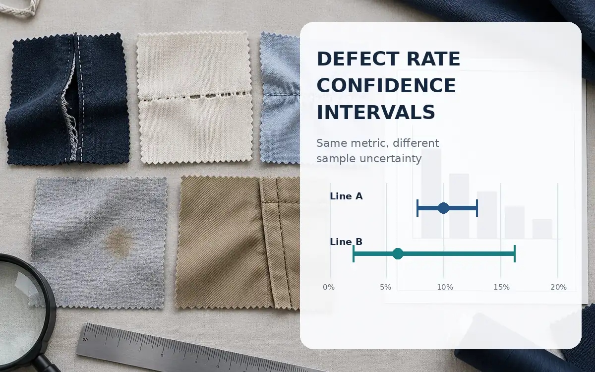
One line reports 10 percent defective from 500 inspected garments; another reports 6 percent from 50. The lower percentage looks better, but the second estimate is based on much less information. A defect rate confidence interval makes that sampling uncertainty visible. This guide uses the Wilson score method for a proportion of defective units, shows a complete calculation and explains why a zero-defect sample, a targeted inspection or a bundle of correlated garments cannot be read as proof of a stable process rate.
Define a defective unit before estimating its rate
For this method, each sampled unit contributes one binary outcome: defective or not defective under a stated criterion. Count a garment once even if it has several faults. The observed proportion is the number of defective garments divided by the number inspected. Keep defect severity and disposition information in the record, but do not let multiple faults on one piece create several binomial trials.
This distinction separates the method from defects per hundred units, or DHU. The site's DHU guide explains why defect observations and defective garments answer different questions. If the log contains only total faults, first recover or collect the defective-unit count. Applying a proportion formula to a count of faults is not a harmless alternative definition.
Write the population or process being described. A result for one style's first-pass end-of-line inspection is not automatically the defect rate of every style, all re-inspected garments or the entire factory. State the date range, stage, criterion and sampling method beside the estimate so the uncertainty calculation is attached to a meaningful operational question.
What the Wilson interval adds
The observed proportion is a point estimate. A confidence interval adds a range produced by a specified statistical procedure under its assumptions. NIST presents Wilson score bounds for a binomial proportion. The method avoids some important failures of the simple normal interval, including an impossible negative lower limit and a collapsed interval when no defects are observed.
A two-sided 95 percent interval refers to a procedure's coverage over repeated comparable sampling. It is not a promise that the next batch will fall inside the range, and it is not a statement that 95 percent of garments conform. Wilson coverage is an approximation whose behaviour depends on the underlying proportion and sample size; Hofer and Held's method comparison discusses evaluating different binomial intervals. Do not describe it as exact coverage for every case.
The arithmetic below uses z = 1.96 as an approximation to the standard-normal quantile for a two-sided 95 percent calculation. Keep the same value throughout the worksheet. A one-sided bound answers a different question and needs a different quantile and interpretation; it should not quietly replace the two-sided interval because it gives a more convenient limit.
Calculate the interval in three steps
Let x be the defective-unit count, n the inspected-unit count and p the observed proportion x divided by n. The following is an equivalent computational description of the Wilson formula. Keep p as a fraction, not a percentage, until reporting the final results. Using 6 where the calculation expects 0.06 is a serious unit mistake.
Calculate the denominator as 1 plus z squared divided by n.
Calculate the adjusted centre as p plus z squared divided by twice n, all divided by that denominator.
Form the sum of p times one minus p divided by n, and z squared divided by four n squared. Take the square root of that sum, multiply by z and divide by the denominator to obtain the half width.
The lower bound is adjusted centre minus half width; the upper bound is adjusted centre plus half width. This description states the full calculation without requiring a particular spreadsheet layout. Keep the intermediate values in the worksheet so a reviewer can distinguish a formula error from an incorrect inspection count.
Consider an illustrative random sample with 12 defective garments among 200 inspected. The observed proportion is 0.06, or 6 percent. With z = 1.96, z squared is 3.8416. The denominator is 1.019208. The adjusted centre is approximately 0.06829224 and the half width approximately 0.03364039.
Calculation item | Value | Reporting meaning |
|---|---|---|
Defective units x | 12 | Each garment counted once |
Inspected units n | 200 | Defined sampling scope |
Observed proportion | 0.060000 | 6.00 percent |
Wilson adjusted centre | 0.06829224 | Intermediate value not observed rate |
Wilson half width | 0.03364039 | Intermediate value |
Lower bound | 0.03465185 | 3.47 percent |
Upper bound | 0.10193264 | 10.19 percent |
Report the finding as 12 of 200 units defective, observed rate 6.0 percent, two-sided 95 percent Wilson interval approximately 3.47 to 10.19 percent. Name the method and scope. Do not replace the observed 6 percent with the adjusted centre; that centre is part of the interval construction, not a new counted defect percentage.
Use a small tested calculation routine
This Python routine requires only the standard library and integer counts. It uses the stated 1.96 approximation and returns fractions. It has been tested on the examples in this article, including zero and all-defective counts. It calculates an interval; it does not validate whether the sampling design makes a binomial model appropriate.
from math import sqrt
def wilson(x, n):
if not isinstance(x, int) or not isinstance(n, int):
raise ValueError("Use integer counts")
if n <= 0 or x < 0 or x > n:
raise ValueError("Require n > 0 and 0 <= x <= n")
z = 1.96
p = x / n
denominator = 1 + z * z / n
centre = (p + z * z / (2 * n)) / denominator
variance = p * (1 - p) / n + z * z / (4 * n * n)
half = z * sqrt(variance) / denominator
return max(0.0, centre - half), min(1.0, centre + half)
print(wilson(12, 200))
For a software implementation using a statistical package, statsmodels documents the Wilson option. Its documented default is the normal method, so the analyst must select Wilson deliberately rather than relying on a generic confidence-interval function name. Check the installed version's API before adopting a package into a production report.
Compare counts before ranking lines
The following rows are illustrative independent sample summaries under a common defective-unit definition. The different sample sizes are intentional. They show why the percentage and the information behind it should be published together.
Sample | Defective units | Inspected units | Observed percent | Wilson interval percent |
|---|---|---|---|---|
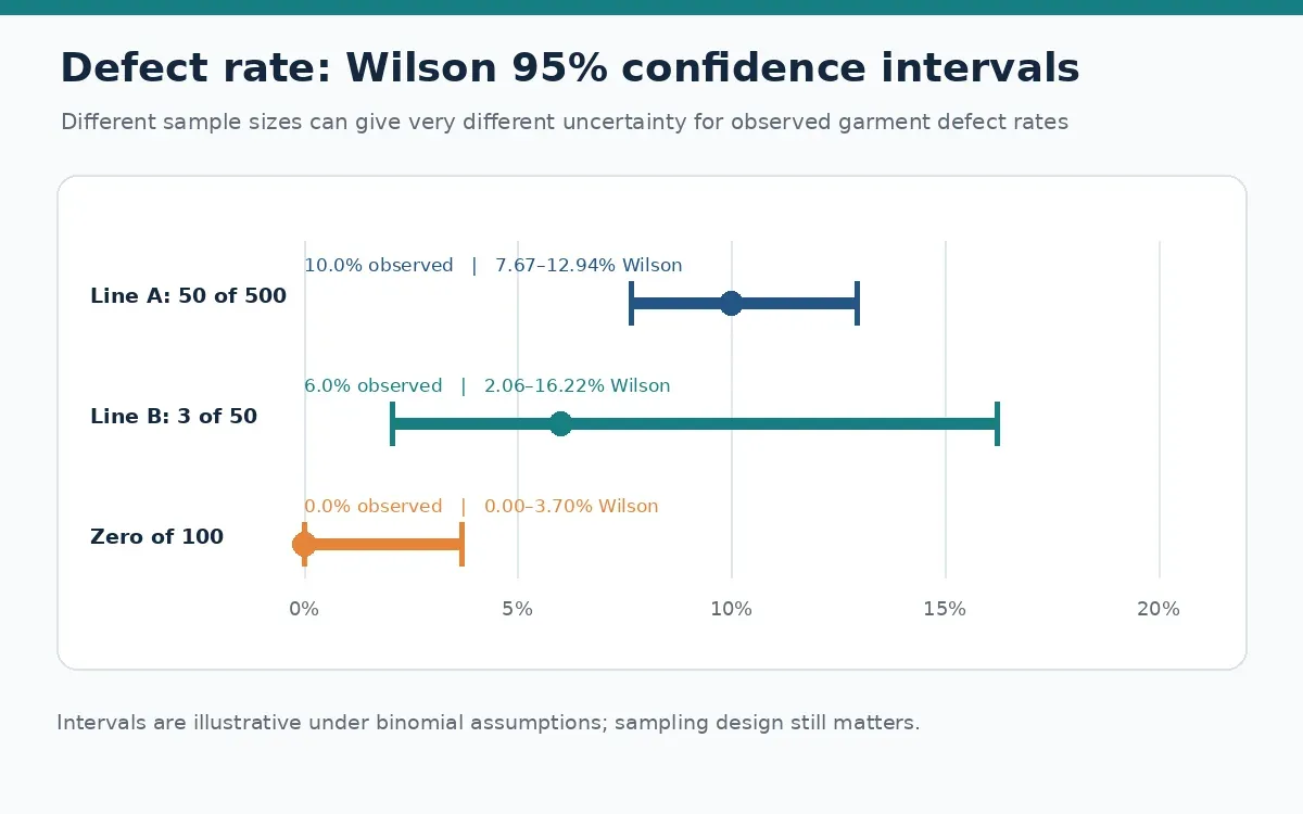
Line A | 50 | 500 | 10.00 | 7.67 to 12.94 |
Line B | 3 | 50 | 6.00 | 2.06 to 16.22 |
Zero-count example | 0 | 100 | 0.00 | 0.00 to 3.70 |
Line B's interval is much wider. The lower point estimate alone is weak evidence for declaring B better than A. Do not treat interval overlap as a formal significance test either: overlap rules can mislead, and a proper comparison must address both the statistical method and whether the lines were sampled comparably. Different garment complexity, defect criteria or inspection targeting can dominate any formula-based comparison.
The zero-count row means no defective units were found in that sample. Its upper bound is approximately 3.70 percent under the stated two-sided Wilson procedure. It does not prove zero underlying risk or grant permission to release a lot against a different acceptance plan. The site's AQL inspection guide concerns acceptance sampling, which is a separate decision framework.
Check the sampling assumptions before acting
A simple binomial model assumes a common underlying probability and sufficiently independent unit outcomes. Garments drawn from one bundle or one short machine episode may share conditions. Targeting visibly difficult pieces can also make a sample unrepresentative. A narrow calculated interval cannot correct those design problems; the analyst needs a sampling plan suited to the population and decision.
If a substantial share of a finite lot is inspected without replacement, seek the appropriate finite-population treatment rather than assuming an unlimited population. If rates change by shift or style, keep useful strata and inspect those changes. For monitoring a process through time, the site's SPC guide addresses control charts; a confidence interval around one pooled rate does not establish process stability.
Publish a rate record people can challenge
Add x, n, inspection scope, selection method, defective-unit definition, confidence level and interval method to the report. Name the person who owns disputed counts. Show missing or zero sample size as no estimate, not 0 percent. A transparent record is particularly useful when management wants to rank lines or claim an improvement from a small change in observed percentages.
Start by adding a Wilson interval to one existing sampled-rate report and reviewing the sample design with QA. Use the wider or uncertain results to decide where more comparable information is needed, while keeping immediate defect correction and buyer acceptance requirements on their own authorised paths.
References
ARTICLE BODY END
Editorial appendix
Content gap: SPC and AQL are covered, but no dedicated sampled-rate confidence interval worksheet was observed.
Distinct added value: Wilson interval with an explicit defective-unit denominator, zero-count example and limitations for clustered or targeted samples.
Nearest existing article: Read existing article
Keyword evidence
Evidence status: Search volume unverified; topic selected using qualitative search-intent and relevance evidence.
Supporting entities and questions: Wilson score interval, proportion defective confidence interval, zero defects sample size, compare production line quality, sample size defect rate, binomial confidence interval; Report uncertainty around a sampled defective-unit percentage and avoid unsupported ranking of differently sampled lines.
Current results assessment: Results focus on statistical derivation or calculators; this article adds defective-unit versus defect counts and real inspection-design limits.
Search-result evidence: https://www.itl.nist.gov/div898/handbook/prc/section2/prc241.htm
Search-result evidence: https://www.statsmodels.org/stable/generated/statsmodels.stats.proportion.proportion_confint.html
Search-result evidence: https://arxiv.org/abs/2207.03199
Evidence limitation: No numerical keyword export, paid-tool access, CPC, difficulty or ranking data. Search-result presence does not prove volume. Unpublished draft history was not supplied.
Source verification
Source 1: https://www.itl.nist.gov/div898/handbook/prc/section2/prc241.htm
NIST formulas read for two-sided Wilson score bounds. z=1.96 approximation is stated and used consistently.
Source 2: https://www.statsmodels.org/stable/generated/statsmodels.stats.proportion.proportion_confint.html
Official statsmodels API read for method='wilson' and alpha=0.05; no reliance on its normal default. Article uses standard-library Python, tested locally.
Source 3: https://arxiv.org/abs/2207.03199
Hofer and Held original research abstract read for method comparisons and limitations. No claim that Wilson has exact 95% coverage for every p,n.
Internal link map
DHU guide: https://appareldiary.com/article/dhu-in-garments-explained-formula-benchmarks-and-why-its-a-profit-metric-part-3 | Define a defective unit before estimating its rate | Explains DHU guide in the linked existing guide or calculator.
AQL inspection guide: https://appareldiary.com/article/aql-2-5-sampling-inspection-practice | Compare counts before ranking lines | Explains AQL inspection guide in the linked existing guide or calculator.
SPC guide: https://appareldiary.com/article/statistical-process-control-practical-guide | Check the sampling assumptions before acting | Explains SPC guide in the linked existing guide or calculator.
Possible backlink: The nearest existing article could link back when this draft is published; no existing page changed.
Pending batch links: See publishing manifest; proposed relationships only until destination articles are live.
Featured image brief
Suggested filename: defect-rate-confidence-intervals-featured.webp
Size and crop: 1200 x 630 pixels; approximately 1.91:1; central 1120 x 630 safe for a 16:9 crop
Generation prompt: Create a clean technical illustration of two garment-inspection sample trays of different capacities. The smaller tray contains a few folded plain garments and the larger tray many smaller simplified garments. Above each tray, show a neutral dot with an unlabelled horizontal interval motif; do not encode numerical confidence bounds, defect rates or relative statistical significance. The image should communicate that sample size affects uncertainty, while all exact labels and bounds are reserved for deterministic plotting after generation. Use a balanced frontal three-quarter viewpoint, smooth white background, soft blue-grey outlines and one muted orange accent. Keep the central trays and interval forms sharp and readable without a legend. Do not depict a real factory result, approve one line, or suggest that an empty defect tray proves zero risk. No people or operating machinery are required. Add natural textile detail without turning the composition into a glossy product advertisement. Deliver at 1200 x 630 pixels, approximately 1.91:1. Keep essential objects inside the central 1120 x 630 crop-safe area for a 16:9 display crop. Use believable proportions and avoid visual clutter. Exclude logos, watermarks, fake certifications, illegible pseudo-text, distorted equipment, implausible hands and unsafe operating practices. Do not depict a named real factory or imply an AI-generated scene documents an actual event.
Draft alt text: Inspection trays of different sizes beside unlabelled interval forms.
Optional caption: Conceptual illustration of two inspection trays of different sizes with simple dot-and-interval forms in an unlabelled technical illustration.
Negative constraints: No logos, watermarks, fake certifications, invented readable data, pseudo-text, distorted equipment, implausible hands, real-factory attribution or unsafe practices.
Confirm technical proportions, equipment state and task-appropriate safeguards. Check central 16:9 crop, compression and small-card readability.
Remove invented labels; manually add any approved text or verified data. Rewrite alt text to describe the actual approved image. Upload the real approved asset and then supply its actual URL.
Human review checklist
Technical review: Verify assumptions and distinguish teaching examples from production settings. Statistician or qualified analyst must validate sampling design, independence, finite-lot relevance and any formal comparison test.
Publishing review: Confirm the topic selection, real author and reviewer identities; recheck links and proposed slug collisions.
Asset review: Inspect the approved image, rights, final alt text and actual uploaded URL.
CMS review: Remove administration before DOCX import or test rendered HTML copying. Complete substantive human review before publication; no ranking, ad-serving or account-approval guarantee.


Discussion0
Loading the discussion…