Rework Loops and Inspection Capacity Calculation

An inspection desk receives 100 new garments an hour, yet its activity log shows 125 inspections. Those figures can both be correct when repaired garments return through the same desk. Counting only first arrivals understates the workload; counting every visit as a new garment overstates throughput. A rework loop needs both a garment count and a visit count.

This guide develops a small capacity screen for inspection followed by repair and reinspection. It shows how repeat visits can move the bottleneck, which records reveal the loop and why a stable workload calculation is different from a prediction of waiting time. The examples are illustrative, with assumptions stated explicitly.

Draw the actual route before estimating capacity

Define where a new garment first enters the system. Identify which outcomes leave the system, which send it to repair and which return it to inspection. Include holds, scrap and alternative routes if they occur. A repair that goes directly to packing has a different workload effect from one that requires another complete inspection.

Use one garment identifier across visits and a separate visit number for each inspection. Record the repair transaction that links the two. Without that relationship, a dashboard may treat the second inspection as another produced garment, or delete it as a duplicate even though it consumed real labour.

The site's queue and buffer guide explains how arrival rates and service capacity affect congestion. Here the missing input is the internal arrival stream created by feedback. A rack sized from first arrivals alone cannot remove that additional work.

Distinguish first pass yield from a repeat routing rate

First pass yield describes the share of original garments that pass without the specified rework. For the simple loop model, q instead denotes the fraction of all inspection visits routed to another repair and reinspection cycle. These denominators coincide only under particular conditions; one should not be silently substituted for the other.

An illustrative closed cohort of 100 original garments makes the distinction visible:

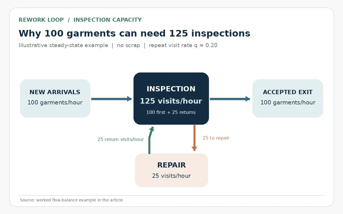
First pass yield is 80 divided by 100, or 80 percent. There are 125 inspection visits and 25 repair visits before the cohort closes. Across all inspection visits, the observed repeat-routing fraction is 25 divided by 125, or 20 percent. The later rounds have few observations; their percentages should not be treated as precisely estimated probabilities.

This cohort happens to reconcile with the simple constant-rate example below. That arithmetic match does not establish that the same routing probability applies to every garment, defect or round. Keep the underlying route counts available.

Use flow balance to expose the hidden workload

Let a be the rate of new garments entering per hour and v the total inspection-visit rate, including returns. Assume every repair returns for inspection, a constant fraction q of inspection visits enters repair, and there are no other routes in the simplified model. In a steady operating state:

Inspection visits = new arrivals + returning repair visits

v = a + q × v, so v = a ÷ (1 − q)

Repair visits per hour = q × a ÷ (1 − q)

With a = 100 garments per hour and q = 0.20, inspection workload is 100 ÷ 0.80 = 125 visits per hour. Repair workload is 0.20 × 125 = 25 visits per hour. The expected visit multiplier is 1.25 inspections per new garment under these assumptions.

MIT's queueing-network lecture distinguishes external arrivals, internal routing and feedback. The calculation here uses flow conservation; it does not assume that all the stronger conditions for a Jackson-network waiting-time model hold on a garment floor.

Check inspection and repair separately

Suppose one inspection resource can perform 150 visits per available working hour, corresponding to 0.40 minutes of service per visit. The repair resource can perform 40 visits per available working hour, corresponding to 1.50 minutes per repair. These are illustrative effective capacity assumptions, not measured industry standards.

At q = 0.20, inspection workload of 125 visits uses 83.33 percent of its 150-visit capacity. Repair workload of 25 uses 62.50 percent of its 40-visit capacity. Use compatible working-time denominators. A repair rate measured only while hands are active should not be compared with arrivals per whole shift without accounting for other required time.

The sensitivity is substantial when the repeat-routing rate rises:

At q = 0.30, the inspection calculation remains below nominal capacity, but the repair requirement exceeds its capacity. Adding inspection capacity alone would miss the constraint. Workload above 100 percent is a warning that the assumed steady operating state cannot be sustained, not a utilisation target to ask people to achieve. MIT's manufacturing-systems queue notes distinguish arrival rate, service capacity and the conditions for a stable simple queue.

Find the capacity ceiling without calling it a safe target

For inspection capacity cI and repair capacity cR, the simple model requires a to be less than both cI × (1 − q) and cR × (1 − q) ÷ q when q is positive. With q = 0.20, those boundaries are 120 and 160 new garments per hour respectively. Inspection is the tighter boundary.

With q = 0.35, the boundaries become 97.5 and approximately 74.29 new garments per hour. Repair is now tighter. At equality the resource has no average spare capacity under the model; variable arrivals, interruptions and changing repair content require additional analysis and operating margin. The mathematical boundary is not a recommended release rate.

For zero repeat routing, repair workload is zero and the division by q is unnecessary. For q approaching one, the workload multiplier grows without bound. A real process should have an authorised disposition and escalation policy, not unlimited repeat repairs justified by a geometric model.

Keep a small route and capacity record

Capture new arrivals, all inspection visits, repair entries, returns, accepted exits, scrap or other exits, and opening and closing work in process. Retain timestamps and service effort where practical. Reconcile counts for a closed cohort or account explicitly for garments still in the loop at the reporting boundary.

The site's DHU explanation deals with defects per hundred units. A garment may contain several defects but create one repair visit, or one defect may generate several unsuccessful visits. Defect counts, defective-garment counts and visit counts therefore answer different planning questions.

Stratify the record by relevant defect and construction. A single average repair time can conceal one repair type using a special machine or skill that other repair staff cannot share. If those routes matter, model separate resources rather than assuming every idle person can perform every repair.

Reconcile the reporting boundary before estimating a return rate

A shift can begin with yesterday's repairs and end with some of today's garments still waiting. Dividing this shift's repair returns by this shift's new arrivals then mixes different cohorts. Keep opening and closing work in process by route, or follow a defined cohort until its final dispositions are known.

Separate a new inspection visit from repeated scans of the same visit. The visit record should have an event identity and a status that distinguishes started, completed and cancelled work. An accidental rescan consumes no additional full inspection service, whereas a genuine reinspection does. Both can look like another row in an unreviewed transaction export.

Also record how service capacity was obtained. A resource's rostered hour may include meetings, necessary checks and other duties, while a measured repair cycle may contain only hands-on work. Use a compatible available-time basis and retain the measured distribution where repair content varies. The flow screen becomes useful only after the route counts and resource denominators describe the same operating scope.

Use the loop analysis to choose the next investigation

First verify whether congestion comes from more new work, more repeats, longer repair content or less available capacity. Each calls for a different response. Inspect the repeated defect and repair method before buying another inspection table. Confirm that a proposed quality intervention actually changes routing or service effort in a controlled trial.

Do not infer waiting minutes from this workload screen. Feedback, batches, priority rules, blocking and variable service times can change queue behaviour. MIT's notes expressly caution that internal feedback arrivals and other performance measures need more careful treatment than independent queue assumptions suggest.

Take the next closed cohort to the planning review with its original garments, inspection visits, repair visits and final dispositions reconciled. Compare that route record with measured capacity for the same scope. The staffing or quality decision can then address the repeated work and constrained resource actually shown by the evidence.

References

• MIT queueing networks lecture on flow conservation routing and feedback.

• MIT manufacturing-systems queue notes on utilisation and stability.