
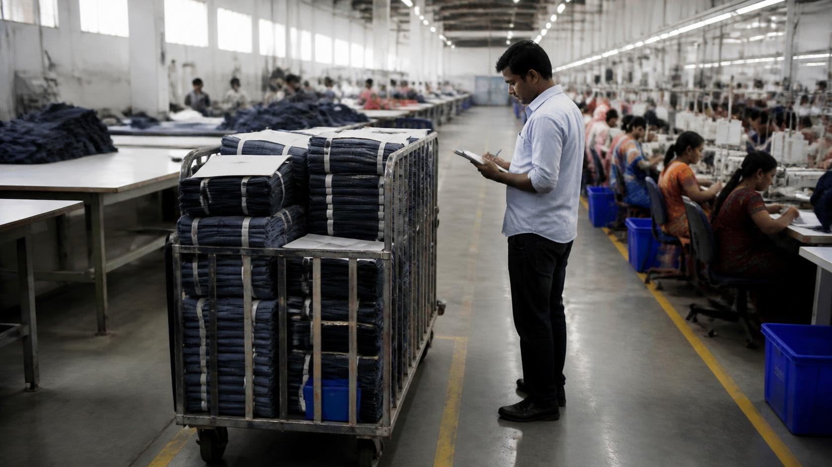
A planner pushes the cutting line to 95% utilisation because the machine cost analysis says idle capacity is waste. Three weeks later the buffer between cutting and sewing has swollen from a tidy 20-bundle rack to a 90-bundle backlog spilling into the aisle.
Nobody changed the demand. Nobody added a shift. The only thing that moved was utilisation, by 15 points, and the queue did not grow by 15%. It grew by nearly 500%.
That gap between "a small change in utilisation" and "a five-fold change in queue length" is the single most expensive misunderstanding in production planning. Most planners treat 90% utilisation as slightly worse than 80%. It is not slightly worse: it is a different regime entirely, and queuing theory buffer sizing gives you the arithmetic to see the cliff before you walk off it.
This article gives you the plain-language version of M/M/1 and M/M/c queues, the utilisation-versus-wait-time table that makes the nonlinearity impossible to ignore, Little's Law as the actual tool you use on the floor, and a worked example sizing WIP buffers between cutting and sewing (the same handoff a kanban pull system between cutting and sewing controls with card counts rather than a formula) and between sewing and finishing, against measured variability rather than gut feel.
What Is an M/M/1 Queue, in Terms a Production Floor Actually Uses?
Strip away the notation and an M/M/1 queue is just: one queue, one server, arrivals that are somewhat random, and service times that are somewhat random. A single sewing machine or a single finishing press, fed by bundles arriving at an uneven rate, is close enough to this model to be useful.
Three numbers drive everything:
Arrival rate (λ): how many units arrive per unit time, bundles per hour reaching the station
Service rate (μ): how many units the station can process per unit time if it never stopped
Utilisation (ρ): the ratio λ/μ, the fraction of capacity actually being consumed
Utilisation is the number that decides everything else, and it is the number most planning meetings treat as a free dial. Push λ toward μ and ρ climbs toward 1. The queue behaviour on the other side of that climb is not linear, and that is the part the rest of this article exists to make concrete.
What Changes When You Add More Than One Machine? (M/M/c)
Most real stations are not single machines: they are a bank of sewing machines, a group of finishing tables, or several pressing units doing the same operation. That is an M/M/c queue: c identical servers sharing one arrival stream.
The practical upside of M/M/c over several separate M/M/1 queues is pooling. A bundle waiting for "any of eight machines" waits less on average than one locked into "this one machine," because an idle neighbour absorbs the spike instead of the load queuing behind a single busy server. Pooling does not create capacity. It reduces the variance the buffer has to absorb, a separate question from how work content is split across those pooled machines in the first place, which is where linear programming for sewing line balancing comes in.
Why Does Utilisation Near 100% Cause Wait Time to Explode?
For a single queue, the standard relationship is that average wait scales with ρ/(1-ρ). Look at what that denominator does as ρ climbs.
Utilisation (ρ) | ρ / (1-ρ) | Relative queue length vs. 70% baseline |
|---|---|---|
70% | 2.33 | 1.0× (baseline) |
80% | 4.00 | 1.7× |
90% | 9.00 | 3.9× |
95% | 19.00 | 8.1× |
98% | 49.00 | 21.0× |
Between 70% and 80% utilisation, queue length grows by less than double. Between 90% and 95%, it more than doubles again, for the same 5-point step. The curve does not rise, it tips over. This is why a planner who pushed utilisation from 80% to 95% for "only" a 15-point gain in machine usage can end up with nearly five times the work-in-progress sitting in front of that station: (0.95/0.05) ÷ (0.80/0.20) = 19/4 = 4.75.
Field note: A knits factory running a single high-speed overlock bank at a chronic 96% utilisation carried a standing WIP buffer of 140 bundles in front of it, with supervisors treating that as "just how that station is." Dropping planned utilisation to 88% by rebalancing two operators onto the bank cut the standing buffer to 38 bundles within nine days, with no change to total daily output: the station had never been throughput-constrained, only queue-constrained by its own utilisation target.
Kingman's Formula: Where Variability Fits Into the Picture
Utilisation alone does not tell the whole story: variability multiplies its effect. Kingman's approximation for average wait in queue is:
Wq ≈ ( (Ca² + Cs²) / 2 ) × ( ρ / (1-ρ) ) × teWhere Ca is the coefficient of variation of arrivals, Cs is the coefficient of variation of service time, ρ is utilisation, and te is the effective mean process time. Read it as a sentence rather than a formula: waiting time is variability times utilisation pressure times process time, and these three multiply rather than add.
Arrival variability (Ca). Batch transfers from an upstream process are the classic driver of a high Ca. Moving cutting-room release from a batch of 50 pieces to a batch of 10 often halves it, smoothing what sewing sees as an arrival stream.
Service variability (Cs). Operator consistency, machine breakdowns, and style changeovers all inflate Cs. Breakdowns do outsized damage here, because they turn a tight, predictable processing-time distribution into a bimodal one: fast most of the time, then a long stall.
Utilisation (ρ). This is the lever with the direct, visible cost attached: an idle machine looks like wasted money in a way that a swollen buffer does not, which is exactly why management pushes it hardest.
Little's Law: The One Formula You Actually Need for Buffer Sizing
Little's Law is the tool that turns all of the above into a physical buffer size you can mark on the floor with tape:
L = λ × WWhere L is the average number of units in the system (your buffer occupancy), λ is the arrival rate, and W is the average time a unit spends waiting. It holds for almost any stable queuing system regardless of the arrival or service distribution, which is why it survives contact with a real, messy factory floor better than the more specific formulas above.
Worked Example: Sizing the Cutting-to-Sewing Buffer
A sewing station processes bundles at 120 pieces per hour. Measured average wait time in the buffer, from arrival to pickup, is 4 minutes.
L = 120 × (4/60) = 8 pieces average buffer occupancy.
An average of 8 is not a ceiling; normal variability means the buffer will run higher than average on plenty of hours across a shift. Size the physical rack for roughly three times the calculated average to absorb normal fluctuation without spilling into the aisle: around 24 pieces, with a hard stop marked at that number.
Worked Example: Sizing the Sewing-to-Finishing Buffer
Finishing and packing typically see higher arrival variability than sewing does, because it inherits every micro-stoppage upstream plus its own changeover pattern. Suppose the finishing table processes 180 pieces per hour, and measured average wait runs 6 minutes.
L = 180 × (6/60) = 18 pieces average buffer occupancy. Applying the same three-times rule gives a working buffer of roughly 54 pieces. Note the buffer needed roughly doubled even though line rate went up 50%, not down, because the wait time it is built on reflects the compounded variability of everything upstream, not just this station's own speed.
Buffer location | Arrival rate | Avg. wait (measured) | Little's Law L | Sized buffer (3× L) |
|---|---|---|---|---|
Cutting → Sewing | 120 pcs/hr | 4 min | 8 pcs | ~24 pcs |
Sewing → Finishing/Packing | 180 pcs/hr | 6 min | 18 pcs | ~54 pcs |
Run this calculation per line and per buffer location, not once for the whole floor. A basic-tee line and a multi-panel jacket line will produce very different λ and W values, and a single floor-wide buffer number will be wrong for both. The order jobs move through those same two stages is a separate decision from how big the buffer between them should be, and Johnson's rule for sequencing jobs across two machines is the tool for that half of the problem.
Where Should You Actually Spend Buffer Space?
Not every station deserves a buffer, and building one everywhere just relocates the WIP problem. Buffers pay for themselves only in two places: immediately in front of the constraint, and immediately after high-variability operations. A simple test decides whether a candidate buffer earns its floor space: if the station downstream never starves without it, the buffer is not doing anything except holding inventory.
Buffer candidate | Keep it if… | Remove or shrink it if… |
|---|---|---|
In front of the bottleneck operation | Downstream starves without it during normal variation | Downstream station is rarely, if ever, waiting |
After a high-breakdown machine bank | Breakdown frequency creates real bimodal service variability | Machine bank has stable, low-breakdown history |
After a style/shade changeover point | Changeovers cluster and create arrival spikes downstream | Changeovers are rare or already staggered |
Between two stably paced stations | Rarely: pooled or balanced stations need little buffer | Almost always: this is where floor space gets wasted |
How Do You Make the Case for 85% Instead of 98% Utilisation?
The arithmetic here is the easy part. The hard part is the meeting where someone asks why you are deliberately planning for 85% utilisation on an expensive machine bank instead of squeezing out every point of capacity you paid for.
The honest answer is a trade: you are buying short, predictable lead times with a small amount of unused capacity. That trade is worth making when short lead time is a genuine commercial advantage. It is a harder sell in a purely price-driven order book, where the utilisation number is what gets reported upward regardless of what it costs downstream in WIP and firefighting. When the underlying question is whether to add capacity rather than just retune utilisation, a decision-tree framework for capacity investment decisions lays that trade-off out formally instead of leaving it to whoever argues loudest in the meeting. Planning for 98% utilisation and firefighting the difference every week costs more, in expediting labour and late-order recovery, than planning for 85% and living inside a buffer sized on purpose.
Buffer Sizing Checklist
Measure actual arrival rate (λ) and service rate (μ) at the station, not the planned rate, the measured one
Calculate utilisation (ρ = λ/μ) and check where it sits on the utilisation-vs-wait-time curve
Estimate coefficient of variation for arrivals (Ca) and service time (Cs) from real shift data
Reduce Ca first if it is high: smaller batch releases upstream are usually cheaper than adding capacity
Measure average wait time (W) at the buffer location directly, not by inference
Apply Little's Law (L = λ × W) to get the average buffer occupancy
Size the physical buffer at roughly 3× the Little's Law average, with a hard, marked ceiling
Apply the starvation test before building any new buffer: does downstream actually starve without it?
Re-run the calculation whenever style mix, batch size, or machine reliability changes materially
Final Word
Queuing theory buffer sizing is not an academic exercise bolted onto a floor that runs on instinct. It answers a question every planner faces weekly: how big should this buffer be, and can I defend that number if someone asks.
Gut-feel buffers drift one way only, bigger, because nobody gets blamed for a rack that is too generous, only for a line that starves. A number built on measured λ, W, and Little's Law is one you can defend, shrink when oversized, and grow on purpose, instead of by accident at 96% utilisation.


Discussion0
Loading the discussion…