Decision Tree Analysis for Capacity Investment Decisions

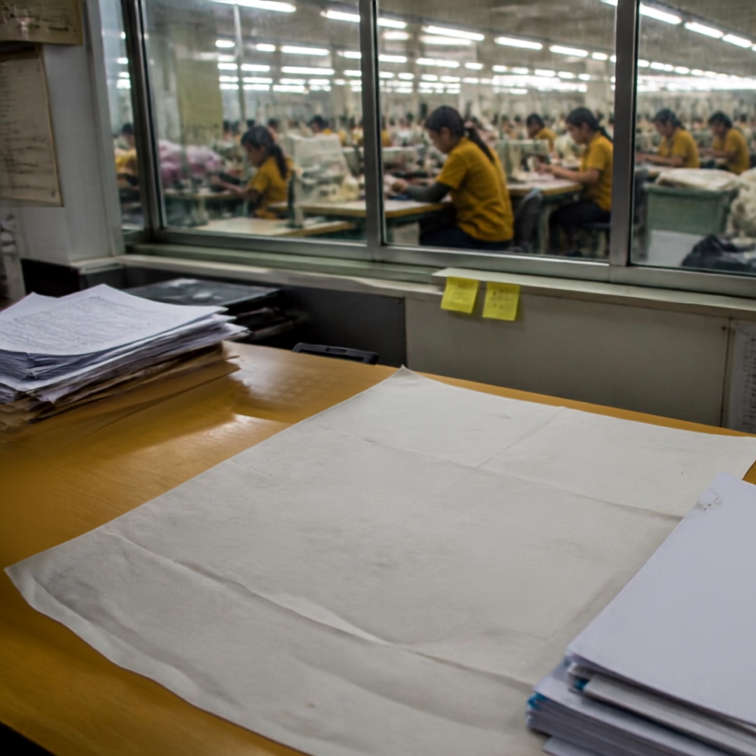
A buyer has just offered you a program that would push volume past your current line capacity. You have three options, a costing sheet, and a Friday deadline to recommend one.

Most factories answer this with a single spreadsheet: one demand number, one payback period, one gut call in the Monday meeting. That single number hides the fact that you are betting capital on a demand forecast nobody can actually guarantee, the same blind spot that shows up when a store picks between EOQ and periodic review inventory policies without checking how unreliable the underlying forecast really is. Get it wrong and the cost is not abstract: a new line sized for demand that does not show up sits half-loaded, eating overhead every month until someone quietly writes it off. A subcontract deal signed because "it felt safer" can also cost you margin for eighteen months if demand turns out strong.

Decision tree analysis forces the uncertainty onto paper before you commit money to it. It will not tell you the future demand number, nothing does, but it will tell you exactly which probability assumption your decision actually depends on, and what you stand to lose if you are wrong.

This article works one capacity decision end to end: add a sewing line, subcontract the overflow, or decline the order. Three demand scenarios, real payoffs, a full expected-value roll-back, and a sensitivity table showing the exact point where the recommended choice flips.

What Is a Decision Tree, in Plant Terms?

A decision tree is a map of choices and uncertainties laid out left to right, in the order they actually happen. A decision node (drawn as a square) is a point where you choose: add the line, subcontract, or decline. You control what happens next. A chance node (drawn as a circle) is a point where the outcome is not yours to choose: which demand scenario actually shows up. Each branch out of a chance node carries a probability, and the probabilities on every branch from one node must sum to 1.0. At the end of each path sits a payoff: the net cash outcome if that decision and that chance branch both happened. Read left to right for the story; solve right to left, the "roll-back" step below.

Field note: A line lead in one Chittagong-area facility used to price capacity decisions on a single "expected" demand figure his merchandiser gave him, never a range. When a buyer's program came in 35% below that figure two seasons running, the new line's payback period doubled and nobody had budgeted for it, because the spreadsheet never showed what happened if the number was wrong.

The Setup: Three Options, Three Demand Scenarios

A regional buyer has offered an 18-month program requiring sewing capacity beyond what the current lines can absorb. Add a sewing line: capex of $180,000 for machines, layout and commissioning sized the way a linear programming line-balancing model would allocate it; adds 40,000 pieces/month of capacity; adds $8,000/month in incremental overhead; in-house margin of $1.30/piece. Subcontract the overflow: no capex; a subcontractor absorbs whatever volume shows up at a lower margin of $0.60/piece, no capacity ceiling. Decline the order: no investment, no incremental margin, no exposure.

Building the Tree and Computing the Payoffs

Draw the decision node first: three branches for Add Line, Subcontract, Decline. From the end of each branch, draw a chance node with High, Moderate, Low branches carrying the probabilities above. Decline needs no chance node, because its payoff is $0 regardless of demand, which is exactly why it belongs in the tree as a real branch, not an assumed baseline.

Each payoff is the 18-month net result for that decision-and-scenario combination. Add Line, net of the $180,000 capex and $8,000/month overhead: High = (40,000 × $1.30 − $8,000) × 18 − $180,000 = $612,000; Moderate = $284,400; Low = –$43,200. Subcontract, no capex, margin of $0.60/piece: High = 40,000 × $0.60 × 18 = $432,000; Moderate = $280,800; Low = $129,600. Decline: $0 on every branch.

Rolling Back the Tree to Expected Value

Rolling back means starting at the payoffs on the right and working left: multiply each payoff by its branch probability, sum across the chance node, and that sum becomes the value of the decision branch feeding it.

On expected value alone, Add Line wins by roughly 4%: $300,780 against $288,360 for Subcontract. That is a thin margin to hang a $180,000 capex decision on, and it is exactly the gap a sensitivity table exists to interrogate.

Before trusting that 4% gap, it is worth asking how much better you could do if the demand scenario were known in advance, the expected value of perfect information (EVPI). Picking the best payoff in each scenario column (High: Add Line $612,000; Moderate: Add Line $284,400; Low: Subcontract $129,600) and weighting by probability gives $343,980. Subtract the $300,780 already identified as best, and EVPI is $43,200, the ceiling on what a market pilot or a phased order commitment would be worth paying for to resolve the uncertainty before committing capital.

Sensitivity Analysis: Where Does the Decision Flip?

The Low-demand probability was set at 0.25 from the merchandising team's scenario plan, a forecast, not a fact. Holding the High:Moderate ratio fixed and varying only the Low-demand probability produces a clean crossover.

The decision flips once the probability of the low-demand scenario rises past roughly 30%, only five points above the base-case estimate. That is the number to defend in the investment committee meeting, not the $180,000 capex figure, and not the headline expected value. If the merchandising team's forecast confidence anywhere near that 30% line is soft, the capital decision is genuinely on a knife edge.

What Expected Value Hides

Expected value is a risk-neutral number. It treats a 25% chance of losing $43,200 as fully offset by the chance of a $612,000 upside, because on paper the weighted average comes out ahead. A factory with thin working capital or a loan covenant tied to monthly cash flow does not experience risk that way.

Add Line's worst case is a $43,200 loss, plus a half-empty line and idle operators if Low demand persists, precisely the over-provisioning risk queuing theory for buffer sizing is built to quantify. Subcontract's worst case is still a $129,600 gain: every demand scenario is profitable, because there is no capex to recover. A factory that cannot survive a $43,200 miss should not take the Add Line branch even if its expected value is higher, because expected value only pays off on average, across many repeated bets, and a single capacity decision is not repeated.

Two other blind spots worth naming before the tree goes into a board pack: sunk costs stay out of the tree entirely: only incremental cash flow from this decision forward belongs in the payoffs. And a staged commitment is a real branch, not a footnote: installing half the capacity now with an option to add the rest once early demand is confirmed is itself a decision node worth drawing.

Checklist: Building a Capacity Decision Tree That Survives Scrutiny

Final Word

A decision tree does not remove the uncertainty in a capacity call; it just stops the uncertainty from hiding inside a single spreadsheet cell, the same failure mode we cover in choosing what to build first in a manufacturing analytics stack. Build the tree, roll it back, then flex the one probability that scares you most before you sign anything.

If the expected-value gap between two options is inside a few percentage points, as it was here, the sensitivity table is the actual decision document, not the EV row. And if the losing branch is one your factory cannot absorb, expected value has already told you everything it can; the rest is a risk conversation, not a math one.