EDD vs SPT Scheduling and Critical Ratio Explained

Four jobs are waiting for the same finishing cell, but the shortest job and the earliest shipment are different orders. A planner needs a rule that matches the decision being made. EDD, SPT and critical ratio are three dispatching methods with different priorities: due date, processing time and urgency relative to remaining work. This guide compares them on one illustrative dataset, explains the measurements behind the comparison and shows how to use a rule without letting it override material readiness or an approved production calendar.

Decide what the cell must protect

Earliest due date, or EDD, puts the job with the earliest due date first. Shortest processing time, or SPT, puts the shortest ready job first. Critical ratio, or CR, divides time remaining until a job's due date by its remaining processing time, then gives the smallest ratio priority. University of Kentucky scheduling notes describe these priority rules. They are easy to calculate; selecting the right performance objective takes more care.

If the purpose is to reduce average time jobs spend waiting and processing, SPT is a useful starting point. If the purpose is to protect against the worst lateness, EDD is a useful starting point. In the equal-release single-machine setting, Berkeley's scheduling resource identifies those respective optimality properties. These guarantees do not extend automatically to changing arrivals, unequal commercial weights, parallel machines or sequence-dependent setups.

Critical ratio is a practical urgency heuristic rather than a general guarantee of minimum tardiness. A ratio below 1 means remaining processing work exceeds the time available before the due date on the chosen time basis. A negative ratio means the job's due date has already passed. A ratio above 1 does not prove the order will ship: other stages, queues, approvals and transport can still consume the apparent slack.

Use one clock and one resource definition

The processing input must describe occupation of the constrained cell, not an unrelated labour-minute total. A garment's standard minute value multiplied by order quantity can estimate labour content, but it does not directly tell you how long one press, packing cell or inspection resource stays occupied. Check machine cycles, batch size, simultaneous work, required operators and any non-overlapping handling. The site's SMV calculation guide helps establish work content; cell occupation needs its own conversion and validation.

Convert buyer shipment dates into an internal due point for this cell. Reserve the downstream time needed for quality release, packing, loading and the actual transport handoff. An order that must leave tomorrow cannot consume all of tomorrow at finishing. Name who approved the internal due dates so an apparent sequencing improvement does not quietly spend another department's time reserve.

For the worked example, time is measured in productive cell hours from the start of the planning window. The approved working calendar converts each internal deadline onto that axis. All four jobs are ready at hour zero, one job occupies the cell at a time, processing cannot be interrupted, and setup time is either absent or already included consistently. Those are teaching assumptions, not descriptions of a factory record.

At the start, EDD chooses B because its due hour is 5. SPT also chooses B because it takes 2 hours. CR chooses A because 8 divided by 6 is the smallest initial ratio. These are different views of urgency, not three interchangeable ways to sort the same column.

Distinguish flow time lateness and tardiness

Completion time is the point at which a job finishes on the chosen clock. Flow time is completion time minus release time. Since all releases are zero here, the flow times equal the completion times. With staggered arrivals, that equality disappears and must not be carried into the next worksheet.

Lateness retains early completion as a negative value. Tardiness counts only the positive delay. Confusing the two can make an average look favourable because several very early jobs cancel one badly late order. The original single-machine study by Hamidi evaluates several distinct objectives, including flow time, delayed-job count and longest delay. State which objective your own review uses rather than calling all of them schedule efficiency.

Calculate the EDD and SPT schedules

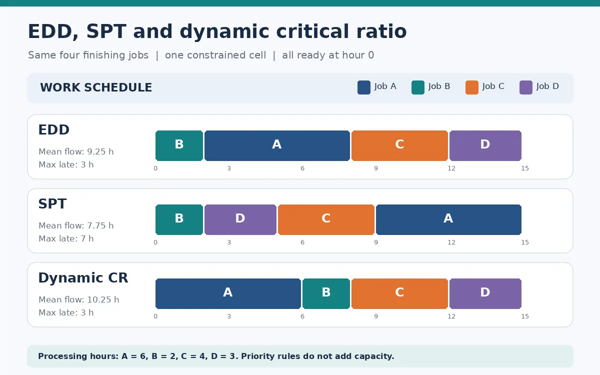
EDD produces B, A, C, D. Completion hours are 2, 8, 12 and 15. Their sum is 37, so average flow time is 37 divided by 4, or 9.25 hours. Job C is 3 hours late; the others are early or exactly on time. Maximum lateness is 3 hours, total tardiness is 3 hours and one job is late.

SPT produces B, D, C, A. Completion hours are 2, 5, 9 and 15, giving a sum of 31 and average flow time of 7.75 hours. Job A is 7 hours late, while C finishes exactly at its due hour. The lower average flow time therefore comes with a worse maximum lateness. It has not created capacity: total processing is still 15 hours under either rule.

The table illustrates why an objective must be named before choosing a rule. If planning reports only average flow time, it will prefer SPT while hiding A's deadline miss. If it reports only the number of late jobs, EDD and SPT both show one, while hiding the different delay lengths. Include the relevant consequence alongside the mathematical score.

Recalculate critical ratio after each completion

Dynamic CR starts with A, which finishes at hour 6. Recalculate the unfinished jobs at that time: B has a ratio of (5 minus 6) divided by 2, or minus 0.5; C has (9 minus 6) divided by 4, or 0.75; D has (15 minus 6) divided by 3, or 3. B therefore goes next even though it is already late. Leaving the initial ratios frozen would answer a different question.

At hour 8, C's ratio is 0.25 and D's is approximately 2.333, so C precedes D. The resulting sequence A, B, C, D has completion hours 6, 8, 12 and 15. Average flow time is 41 divided by 4, or 10.25 hours. B and C are each 3 hours late, so total tardiness is 6 hours and two jobs are late. CR ties EDD on maximum lateness in this example but loses on the other reported measures.

Do not infer from that one example that CR is always worse. It shows why a heuristic needs a trial against the objective and actual operating conditions. Equally, an urgency score cannot repair a missed deadline by itself. If every remaining job has a ratio below 1, the planner must examine capacity, alternatives and customer commitments rather than arguing about the sort order.

Gate the dispatch list before releasing work

Create a ready queue that contains only jobs whose material, approval and equipment prerequisites are satisfied. An unavailable job may remain in the planning backlog, but it should not block a physically ready job merely because its due date is earlier. Record the blocked reason and its owner. Keep a clear distinction between ranking ready work and resolving the causes that prevent readiness.

For significant changeovers, calculate the consequences of the proposed sequence with the relevant setup times. Do not hide a colour change or tooling replacement inside an average processing time if it depends on the predecessor. For two stages with fixed order and the right assumptions, consult the site's Johnson's rule guide. That makespan problem is different from the due-date decision in this article.

A simple dispatch record should include job identity, ready time, validated cell hours, internal due time, setup requirement, selected rule, computed score, chosen position and any approved override. The supervisor owns execution, the planner owns the sequence and due assumptions, and the equipment owner confirms constraints. Agree tie-breaking in advance, such as earlier due date followed by a stable job identifier, so the list can be reproduced.

Run a controlled comparison

Start with a completed planning window and replay EDD, SPT and dynamic CR on the same validated jobs. Report flow time, maximum lateness, total tardiness and late-job count together, then identify which measures matter commercially. In this example, total tardiness is 3, 7 and 6 hours respectively. The best rule depends on the objective; no ranking removes the need to check resource feasibility.

Next run a supervised pilot on one cell with a recorded override reason whenever the published list changes. Review whether the failure came from the dispatch rule, inaccurate times, a changed deadline or an unready order. That distinction gives planning a useful next action and prevents a bad input record from being mistaken for a bad scheduling method.

References

• Berkeley RIOT scheduling algorithms.

• University of Kentucky priority-rule notes.

• Hamidi, Two New Sequencing Rules for the Non-Preemptive Single Machine Scheduling Problem.