
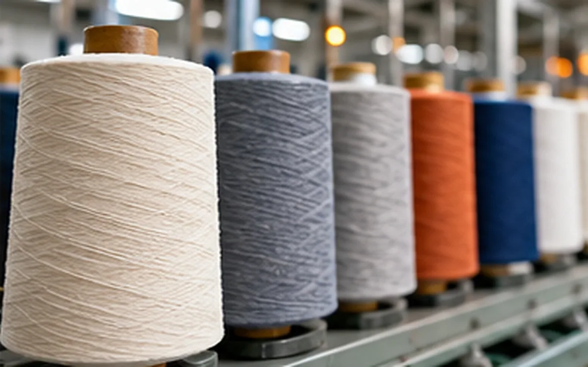
Begin with the shape of the fault
A yarn can meet its average count and still contain a repeating thick place. Another yarn may have no clear repeat but show wide, uneven swings in mass. Both need attention, yet they call for different checks. To investigate drafting irregularity, follow the material through each spinning stage. Track where its mass variation changes.
The useful question is where a particular fault first appears, grows or changes shape. A high final yarn CV does not answer that question by itself. Neither does a tall peak on a spectrogram. Each result needs a test basis, a location in the process and a possible physical explanation.
This guide uses roller drafting as its main setting. All the worked cases below are invented. They explain the principles but do not set mill benchmarks or machine settings. They help separate uneven feed from faults added in processing. They also show how the test itself can affect a result.
Keep average count and evenness separate
Linear density describes mass per unit length. Evenness describes how that mass changes along the strand. A small spread around the wrong average can still produce an off-count product.
Suppose the target sliver is 3.00 ktex. One trial gives a mean of 3.00 ktex and a CV of 2.0%. A second gives 3.10 ktex and a CV of 1.5%, measured on the same basis. The second trial is more even, but its mean is 3.33% above target:
Mean error = (3.10 − 3.00) ÷ 3.00 × 100 = 3.33%.
That result does not justify accepting the heavier sliver. It shows why the mean and its spread belong on separate lines in the report. ApparelDiary’s yarn count conversion guide explains the different count systems. For the examples here, 1 ktex equals 1 gram per metre.
To find the coefficient of variation, divide the standard deviation by the mean. Express that ratio as a percentage. Use the same measurement method when comparing CV values. Weighed lengths describe mass over a chosen distance. An instrument’s short-zone signal may cover a different range of variation.
ASTM D1425/D1425M covers unevenness measured by capacitance. It applies to strands such as sliver, roving and yarn. Its public guidance lists conditions needed for comparison. These include test length, sensing-zone length, speed, preparation and atmosphere. Fibre types can differ in their electrical properties. An uneven blend of such fibres can affect the signal, so check the blend as well as its mass.
What the drafting zone changes
Roller drafting makes a strand finer by allowing fibres to move past one another. The delivery rollers move faster than the feed rollers. Fibre movement must remain under control. Each fibre does not stretch by the full draft ratio.
Between the roller nips, some fibres lack direct grip at either end. Their movement depends on contact with nearby fibres and control surfaces. Groups may accelerate at the wrong point. The outgoing strand can then alternate between heavier and lighter regions. Errol Wood’s roller-drafting teaching chapter explains these floating-fibre and fibre-control principles. Do not transfer its wool setting ranges to cotton equipment.
Fibre length alone does not fully describe this behaviour. Preparation, fibre shape and the way fibres lie in the strand also matter. A nominal setting that worked on one feed may give a different result after the material changes.
Research by Shen and colleagues examined where floating fibres accelerate in roller drafting. Their published abstract describes a method that uses tracers. It also reports a link with output variation. This supports work on fibre movement, but it gives no universal setting recipe. Spacer, pressure and roller distance still need a basis suited to the line.
Treat those settings as a combined system. A change in one setting can alter fibre control elsewhere. Changing several at once makes a trial hard to interpret.
Check the mass-flow calculation first
Check whether the feed, draft and output count agree before seeking a subtle fault. Look for missing feed ends and wrong count conversions first. A detailed spectrogram study cannot resolve those basic errors.
Consider six slivers, each at 5 ktex, entering together at 80 metres per minute. Their combined linear density is:
Combined feed = 6 × 5 = 30 ktex, or 30 g/m.
If the delivery speed is 480 metres per minute, the ideal speed draft is:
Draft = 480 ÷ 80 = 6.
Assume steady flow, no material loss and no change in the stated mass basis. The expected delivery is then:
Output linear density = 30 ÷ 6 = 5 ktex.
The flow check gives the same answer from both sides:
Feed: 30 g/m × 80 m/min = 2,400 g/min.
Delivery: 5 g/m × 480 m/min = 2,400 g/min.
The six feed ends matter. Use their combined count in the calculation. Using just one feed sliver would wrongly suggest a draft of one.
This balance assumes steady flow. Each short section need not follow ideal roller motion. Measured material draft can differ from surface-speed draft. Slip, relaxation, waste and moisture changes can all play a part. Record those effects; do not adjust a figure just to make the balance look right.
Mass conservation also forms part of Komori and Itoh’s theoretical treatment of roller drafting. Their model describes bundle motion and how fibres interact. It is not a machine acceptance test. The simple balance above is a practical first check within its stated assumptions.
Understand what doubling can average out
Combining slivers can reduce variation when their thick and thin sections do not coincide. The benefit depends on how the feeds relate to one another. The number of cans at the creel is only part of that picture.
Take four equal-mean slivers, each with a CV of 4%. In an ideal statistical model, their local mass changes are independent. Combining them gives:
Combined CV = individual CV ÷ square root of feed count.
Combined CV = 4% ÷ square root of 4 = 2%.
This is an averaging calculation before allowing for new variation from drafting. It is not a promised draw-frame result.
Now suppose all four feeds are 10% heavy at the same point. Their combined mass is also 10% heavy. Four matching errors do not cancel merely because four cans are present.
There is a useful middle case. If four feeds have equal means and equal CVs, and every pair has correlation 0.5, the combined CV is:
4% × square root of [(1 + 3 × 0.5) ÷ 4] = 3.16%.
Here, correlation describes how strongly the local changes move together. The result sits between independent feeds at 2% and perfectly matching feeds at 4%. The stated correlation must apply to every pair of feeds. It must also hold at the length scale being compared.
The practical lesson is to record where the feed cans came from. Several cans from one earlier fault episode may carry related variation. Calling them separate feeds does not make their errors independent.
Also ask how the cans were sampled. Short samples in sequence from one can show local changes. Samples spread across several cans may reveal a different feature. Keep the sample plan consistent when judging whether doubling helped.
Read the trace before naming the cause
Start with the mass diagram. Does it show isolated events, gradual drift, repeated oscillation or a mixture? Then use the spectrogram to examine the wavelengths that contribute to the variation.
A narrow peak suggests a repeat worth tracing. A broader raised region suggests variation spread across a range of wavelengths. These are observations about the signal. They do not, by themselves, identify a particular roller or prove that all variation came from drafting. An early ATIRA study of yarn spectra develops this distinction between periodic and broader variation. Its theory is useful here; its older equipment details are not current instrument instructions.
Modern instruments can provide several views of the same test. The Uster Tester 6 technical data lists mass CV, different length-based CV values, diagrams and spectrograms. Each view answers a different question. A single overall CV can conceal a clear repeat that occupies only part of the signal.
Check whether the event is present in several packages. A peak from one short test may deserve a repeat test before anyone changes a setting. If a fault appears only near a package start or end, preserve that location information.
Review the test trace for handling events too. Was the sample disturbed or prepared in the wrong way? Did the test stop? These details may help explain a feature. Keep the original trace so another person can see the basis of the diagnosis.
Convert a wavelength into a testable hypothesis
Imagine a repeat created once per revolution of a roller with a diameter of 32 mm. Its circumference is:
Circumference = π × 32 = 100.53 mm, or 0.10053 m.
Suppose a fault enters the strand at that location. It later passes through a draft of 40. Its ideal downstream wavelength becomes:
Wavelength = 0.10053 × 40 = 4.02 m.
The 4.02-metre prediction assumes one event per revolution and uniform subsequent extension. The relevant draft is the draft after the fault enters the material. It is not automatically the total draft displayed for the whole machine.
This calculation creates a candidate to investigate. It does not establish that a 32-mm roller caused an observed four-metre peak. A different part, two events per revolution or another periodic disturbance could give a similar result. Wood’s teaching chapter also discusses recurring mechanical faults and their relation to roller motion.
A time-based disturbance can produce the same spacing. Suppose material moves at 24 metres per minute where a disturbance occurs every ten seconds:
Speed = 24 ÷ 60 = 0.4 m/s.
Spacing at that point = 0.4 × 10 = 4 m.
If the material is drafted again, apply the later draft to this spacing too. The example shows why both part motion and process timing belong in the investigation.
Record a predicted wavelength before inspecting a candidate part. Compare it with the measured feature. Then seek evidence that can separate the possible causes. A repeat may be linked to one machine position, for example. That offers more evidence than a wavelength match alone.
Make sure the test length can reveal the feature
A 100-metre test contains 25 repeats of a four-metre fault. It contains only 2.5 repeats of a forty-metre fault. Both tests cover the same total length, but they offer very different evidence about a stable recurring pattern.
There is no single repeat count here that guarantees a valid diagnosis. Use the instrument’s method and a test length suited to the question. For long variation, include package or can sampling that can capture the relevant distance. Repeating a short test at the same location does not extend its view of the material.
Link samples through the actual material route
Use material that truly passed through the stages being compared. A sliver sample taken this morning may have no link to yesterday’s yarn packages. A shared blend code does not establish that link.
For a limited study, identify the incoming cans, the delivered can, the roving bobbins and the final yarn packages. Record the route, machine positions and changeover times. Allow for material already inside each machine and for cans waiting between stages.
There are three possibilities to distinguish. A feature may travel with the feed, appear at one processing position, or change with both. A controlled comparison can help separate them.
The following invented results use the same yarn count, twist and laboratory conditions. Each cell represents a planned set of samples, not a single short reading.
Feed group | Processing position P | Processing position Q | Initial observation |
|---|---|---|---|
A | CVm 13.1% | CVm 15.3% | Q gives higher variation |
B | CVm 13.0% | CVm 15.1% | The same position pattern returns |
These results justify closer work on position Q and its test trace. They do not prove a worn cot or exclude a common operating difference. Review sample handling, the environment and the test sequence too. Could any of these explain the pattern?
If both positions worsened only with feed B, examine that feed next. Study how it behaves in the process. Mixed results may require a wider study. Avoid forcing an uncertain result into a simple feed-versus-machine conclusion.
Any planned material exchange must follow the machine’s operating procedure. Keep the settings and sample identities traceable, and use qualified staff for machine inspections. Changes made during a running trial can otherwise destroy the comparison.
Do not subtract CV values to measure an added fault
An incoming CV of 2% and an outgoing CV of 3% do not show that a machine added exactly one percentage point of variation. CV describes a spread relative to a mean. It is not a quantity that can always be split by simple subtraction.
Under a narrow model, independent relative variations add through their variances. If the signals have compatible definitions and the incoming variation passes through unchanged, an added component would be:
Added CV = square root of (3² − 2²) = 2.24%.
This calculation explains the assumption. It cannot diagnose a line without further evidence. Correlation, levelling and changes in fibre movement can all break the model. The compared lengths also need to represent the same material scale after draft.
A first report should state what was measured at the input and output. Give the definitions, values and sample locations, then describe changes in the trace. If a model estimates added variation, put its assumptions beside the result.
For repeat production, ApparelDiary’s statistical process control guide explains how a stable baseline supports decisions about change. Control limits describe process behaviour; they do not replace the product’s quality requirements.
Check levelling timing and machine condition
An autoleveller must act on the material section that produced the measurement. The sensing point and the point where draft changes take effect are separated by a material path. A timing error can make the correction act too early or too late.
Rieter’s draw-frame brochure describes feed scanning, the levelling action point and independent delivery monitoring on the featured machines. It also describes automatic action-point setting. Those details are model-specific; use the applicable machine instructions when checking them.
Consider a simple timing example with a 0.6-metre path. Assume the material moves at 60 metres per minute throughout. The speed is 1 m/s, so the travel time is 0.6 seconds. A delay error of 0.1 seconds means an error of 0.1 metre along this assumed path.
Real drafting paths need not have one constant material speed. This calculation explains timing. It does not give a delay to enter on the machine. Follow the procedure for the actual measuring and drafting system.
Physical condition also belongs in the review. Rieter’s 2024 draw-frame maintenance case identifies belts, cots and scanning or clearing components in a refurbishment package. The reported results concern that customer’s polyester process. They do not establish a universal replacement interval or a guaranteed quality gain.
For the machine under study, compare its condition with the maker’s limits. Record the part and position, the evidence found and the work completed. A statement such as “drafting checked” is too vague to connect a repair with a later change in the trace.
Report imperfections without losing their test basis
Imperfection counts complement CV, but their meaning depends on the thresholds used. A report must state the thin, thick and nep settings, the tested length and the yarn route. Uster’s technical sheet, for example, distinguishes standard ring-yarn settings from other threshold choices and spinning systems.
Suppose a 500-metre test records 15 thin places, 40 thick places and 25 neps under declared settings. The total is 80 events, giving:
Total imperfections per kilometre = 80 ÷ 500 × 1,000 = 160/km.
The separate rates are 30 thin, 80 thick and 50 nep events per kilometre. Keep them separate as well as reporting the total. A falling total can hide a rise in one important category.
These events are classes defined by the instrument. They do not directly count defective garments or reveal the origin of each event. If nep events drive a complaint, examine the material and the defect itself. The count alone cannot establish a cause.
When test lengths differ, compare rates on a common basis and retain the actual counts. A short sample with ten events may give the same rate as a much longer sample. Yet the uncertainty around each rate can differ. Avoid declaring a reliable improvement from a small rate change alone.
Separate fault-finding samples from production estimates
Samples selected to reveal a fault are useful, but they may not represent its frequency in the whole lot. Keep those two purposes separate when planning the test and writing the result.
Suppose a team suspects problems near joins. It selects 200 metres of material around known joins and records 24 qualifying events. The rate within those selected sections is:
24 ÷ 200 × 1,000 = 120 events/km.
That is a valid description of the sections tested. It is not automatically the average rate across all production. Imagine that the sections belong to a 10,000-metre lot that has been tested in full. Assume the remaining 9,800 metres contain no events under the same definition. The lot rate is then:
24 ÷ 10,000 × 1,000 = 2.4 events/km.
The two rates answer different questions. The selected samples help locate a join-related concern; the full-lot result estimates its overall frequency. In practice, the remainder may not be event-free or fully tested. Do not assume either condition from the selected sample alone.
To find a cause, retain the join or restart location. Compare it with nearby steady-running material. To estimate a production rate, sample across the lot’s material and package locations. If both studies run together, label their results clearly. Do not use the concentrated fault search to estimate the whole lot’s rate.
The reverse problem is also possible. A routine sample from the middle of each package can miss a fault confined to package starts. A good average then says little about the affected region. The complaint should guide an extra targeted check, while the routine plan continues to serve its original purpose.
Confirm the cause through the result
Close the investigation with a prediction. If a specific fault caused the repeat, what should change after the corrective work? Name the wavelength, the affected positions and the test conditions before reviewing the new result.
Then check the mean count, the relevant CV values, the trace and the imperfection categories. Retest enough material to cover the previously affected package locations. Include downstream performance where it drove the original concern, such as repeated yarn breaks or a visible fabric pattern.
A better average CV with the same damaging repeat is an incomplete result. A vanished peak with a new count error also needs further work. The strongest conclusion connects the observed fault with a plausible physical cause. A controlled correction should produce a repeatable change.
Keep unresolved findings visible. Drafting irregularity often reflects both the incoming material and the conditions under which fibres move. A clear account of what remains uncertain is more useful than a confident cause that the evidence cannot support.
References
ASTM D1425/D1425M-14(2020): unevenness of textile strands by capacitance testing. Public scope and comparison guidance; the complete paid method was not used.
Wood: Roller Drafting, Australian Wool Education Trust teaching resource. Basic fibre-control and drafting principles, with a wool-specific context.
Shen and colleagues: measuring the accelerated point of floating fibres in roller drafting. Public research abstract.
Komori and Itoh: A New Approach to the Dynamics of Roller Draft. Theoretical model; public abstract.
Narasimham, Ganesh and Kothari: A Theoretical Study of Yarn Irregularity through the Spectrum. ATIRA research published in 1976.
Uster Tester 6 technical data, April 2026. Instrument outputs and test-setting definitions.
Rieter draw-frame brochure. Sensing, levelling and monitoring on the described equipment.
Rieter: Draw Frame Mini Kit Improves Sliver and Yarn Quality. Manufacturer’s maintenance case, November 2024.

Discussion0
Loading the discussion…