Factory Peak Demand Analysis from Interval Meter Data

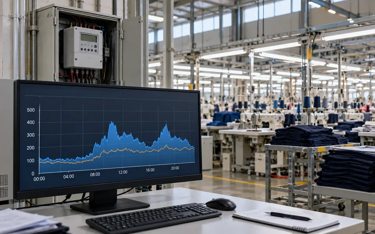
Find the interval that sets the bill

A factory can use less electricity during a month and still pay the same demand charge. It can also lower that charge while using almost the same number of kilowatt-hours. The difference lies in when the load runs and how the tariff measures demand.

Factory peak demand analysis starts with time-based meter data. It asks which loads overlap during costly intervals, which work can move, and whether the change lowers the billing peak. A list of machine ratings cannot answer those questions on its own.

This guide shows how to clean interval records, calculate demand, test a new schedule, and verify the result. The examples describe a hypothetical garment factory. All prices and load figures are teaching assumptions. Actual billing rules must come from the factory's tariff and meter setup.

Use the factory utility load register to locate major loads and their supply points. Then link those assets to measured events. This analysis concerns the operating pattern at the billing meter, not the size of equipment to purchase.

Separate energy, demand, and billed demand

Energy is the amount of electricity used. It is commonly measured in kWh. Demand is the rate of use, measured in kW when the tariff uses active power. Billed demand is the value to which the tariff applies its demand rate.

These values need not move together, as a simple example of a 40 kW load shows. Running that load for half an hour uses 20 kWh. Moving that work to a later half hour keeps the same energy in an ideal case. It may lower the factory peak if the later period has enough spare capacity.

The tariff may use kVA instead of kW, and it may also include power factor terms, several time windows, or a minimum demand. Confirm the unit before building the model. A spreadsheet headed only “load” is too vague.

The U.S. Department of Energy's tariff guide distinguishes energy, demand, and fixed charges. Use those categories to map the bill. A load shift may affect one charge and leave the others unchanged.

Make a one-page billing note with the rate name, effective dates, meter boundary, demand interval, and charge formula, then record who checked it. Update that note whenever the tariff changes.

Convert interval energy into average power

First identify what each meter row contains. It may show energy used during an interval, average power, or a cumulative energy register, and these require different treatment.

For interval energy:

Average demand in kW = interval energy in kWh / interval length in hours

If a 15-minute interval contains 62 kWh, average demand is:

62 / 0.25 = 248 kW

Multiply 15-minute kWh by four to obtain kW. Do not multiply a field already expressed in average kW. For cumulative readings, first take the difference between valid consecutive readings. Handle a meter reset or rollover before using that difference.

The Bonneville Power Administration demand measurement guide highlights this unit distinction. It also explains why the timestamp convention matters. A row labelled 09:15 may describe 09:00–09:15, rather than the next quarter hour.

Place the start and end time in separate columns during analysis to avoid confusion when a supervisor checks a machine start against the meter record. Keep the source timestamp as well, so every change can be traced.

Match the meter's demand window

A fixed block meter may calculate one average for 09:00–09:15, then another for 09:15–09:30. A rolling method can update a 15-minute average every five minutes. Both use a 15-minute length, but they can report different peaks.

Schneider Electric's meter manual describes fixed and rolling block methods. The setting is part of the measurement definition. Match the utility method when estimating a charge.

Consider these hypothetical five-minute average loads:

The two fixed quarter-hour averages are both 233.33 kW. Yet the rolling average for 09:05–09:20 is 366.67 kW. The next rolling window has the same value.

A chart using only the two fixed blocks hides this higher rolling peak. Avoid trying to shift a load just across a clock boundary without knowing the meter method.

BC Hydro's guidance gives a real example of 15-minute demand built from five-minute subintervals. That is a useful illustration, not a rule for every utility or factory.

Do not confuse a short spike with billing demand

A high instantaneous reading may matter for equipment and power quality. It does not necessarily equal the billing demand. An interval average weights the load by how long it lasts.

Suppose a hypothetical circuit draws 600 kW for one minute. It draws 200 kW for the other fourteen minutes. Its 15-minute average is:

(600 × 1 + 200 × 14) / 15 = 226.67 kW

The 600 kW peak may require an electrical investigation. For this assumed demand calculation, however, the interval contributes 226.67 kW. Reporting 600 kW as the tariff peak would overstate the billing effect.

Use separate records for short electrical events and billing intervals. A slower energy logger may be suitable for bill analysis but miss voltage sags or fast current events. The instrument and sampling method should fit the question.

Clean the data before ranking peaks

Keep a raw export that remains unchanged. Work on a copy and add a quality flag to each row. A suspicious value should trigger an investigation of its source, rather than automatic deletion from the record.

For a complete 30-day period with 15-minute records and no clock change, expect 2,880 intervals. That is 30 × 24 × 4. A different count needs an explanation. Possible explanations include differences between billing dates and export dates, another demand interval setting, or missing records.

Check duplicate timestamps, gaps, negative values, meter changes, and repeated flat readings. Confirm time zone and daylight-saving treatment where applicable. Check whether current and voltage transformer multipliers are already included. Applying a multiplier twice can inflate the whole profile.

Reconcile the sum of interval kWh with the bill or a matching register difference. Use the same dates and boundary, because differences can arise from estimated billing, import and export treatment, or a missing day. Explain it before using the peak.

Do not fill a missing high-load period with the monthly average and then call the maximum verified. The missing period may contain the actual peak. Label the result incomplete until the record or an independent check resolves it.

Build three views of the load

Start with a time plot. It shows when the load rises and how long each event lasts. Add shift changes, production starts, planned stops, and known faults. This helps the team connect a pattern to real work.

Next, sort interval demand from highest to lowest. This load duration view shows whether the peak is rare or sustained. PNNL's metering guide uses this method to assess demand reduction opportunities.

Finally, make an event table for the highest intervals. Include the date, load, major equipment status, and a short explanation. Separate evidence from guesses. “Dryer started at 09:12” is stronger than “probably finishing.”

An average daily curve is helpful for routine patterns. It can hide the one unusual day that sets the bill. Keep the maximum-event view beside the average view so the team can distinguish exceptional events from routine operating patterns.

If the highest intervals occur on many days, one start-up change may have limited value. If they cluster around one repeated overlap, a simple schedule trial may be worthwhile. The shape tells the team where to investigate next.

Check which loads overlap

The factory peak is the sum of loads at the same time and boundary. It is not the sum of each department's separate maximum.

Suppose sewing peaks at 150 kW, finishing at 120 kW, and utilities at 110 kW. Adding those maxima gives 380 kW. But at the factory's highest interval, the three readings may be 150, 80, and 100 kW. Their coincident sum is 330 kW.

The separate maxima remain useful for local equipment checks, but they do not prove a 380 kW service demand. Synchronize submeter clocks before making the comparison.

Also account for unmetered loads and losses between boundaries. If the submeter sum differs from the main meter, investigate the gap. Do not assign it to a convenient department without evidence.

Use a short list of likely contributors. Measure them during the critical intervals. The aim is to find controllable overlap, not install a meter on every small machine before taking any action.

Use load factor with the right time base

The U.S. Energy Information Administration defines load factor as average load divided by peak load over the stated period. For interval records at one boundary:

Load factor = total kWh / (peak kW × hours in the period)

Suppose the factory uses 144,000 kWh in a 30-day month. Its measured peak is 400 kW. The calendar period contains 720 hours, so:

Load factor = 144,000 / (400 × 720) = 0.50, or 50%

If the same energy is used with a 360 kW peak, load factor becomes 55.56%. The flatter profile uses the available demand capacity more evenly.

Do not replace 720 calendar hours with production hours while keeping the same monthly energy and peak. That creates a different metric. It may be useful, but it needs a clear name and boundary.

A higher load factor is not proof of lower energy use. Leaving unnecessary equipment on at night can raise average demand and the ratio. Always review kWh, peak demand, and production performance together.

Test a shift with a complete load balance

Assume a flexible 40 kW task runs from 09:15 to 09:45. Production confirms it can move to 10:00–10:30 without delaying the next process. The example assumes the same power and duration after the move.

Subtract the task from its original intervals. Add it to the new ones. Then recalculate the highest demand across the entire billing period.

The six intervals use 505 kWh before and after the shift. The shown peak falls from 400 to 360 kW. This is a demand reduction with no energy reduction under the stated assumptions.

Now check every other interval. If an unchanged event still reaches 380 kW, the monthly peak falls only to 380. If another event remains at 400, the demand charge may not fall at all.

This is why a successful trial on one day cannot establish the monthly saving. The plan must control every event that would otherwise set a higher peak.

Translate the revised peak into money

Assume the whole-month review confirms a drop from 400 to 360 kW. A hypothetical tariff charges 14 currency units per kW per month. It has no minimum demand or look-back rule.

Demand benefit = (400 − 360) × 14 = 560 currency units that month

The energy charge stays the same if total kWh and energy prices remain unchanged. If the task moves between different energy price periods, calculate that effect separately. Include any extra warm-up energy or paid labour caused by the move.

Now add a hypothetical tariff floor equal to 80% of a previous 500 kW peak. The floor is 400 kW. Billed demand remains 400 kW even though the present measured peak falls to 360. The immediate demand-charge benefit is zero.

This look-back rule is often called a ratchet. Its percentage, look-back period, and application vary. Use the actual formula. A lower current peak may still help future periods after an old high value expires, but model those months explicitly.

Where a bill has both all-hours and on-peak demand charges, calculate each maximum separately. A shift can lower one charge and raise another. Review the total bill effect before calling the action successful.

Worked example with two demand charges

Consider a second hypothetical tariff that applies two charges together. The all-hours demand rate is 14 currency units per kW. A separate charge of 6 per kW applies to the highest interval within a defined on-peak window.

Before the schedule change, assume the all-hours maximum is 400 kW and the on-peak maximum is 340 kW. Those maxima occur at different times. The demand portion of the bill is:

400 × 14 + 340 × 6 = 7,640 currency units

The proposed shift lowers the all-hours maximum to 360 kW, but it moves work into the on-peak window. The new on-peak maximum becomes 350 kW. The revised demand cost is:

360 × 14 + 350 × 6 = 7,140 currency units

The net demand benefit is 500. Looking only at the all-hours reduction would predict 560 and overstate the saving by 60. Looking only at the on-peak increase would miss the larger overall benefit.

This example assumes both charges apply and that no floor or other adjustment changes them. It shows why each tariff component needs its own calculation, followed by one combined comparison. Preserve the time labels when building that comparison; sorting the demand values alone would lose the information needed to assign each interval to its billing window.

Protect process needs when choosing flexible loads

Some tasks can move within a defined scheduling window, while others must run when the process needs them. Do not classify a load as flexible just because a switch can turn it off.

For each candidate, record its earliest start, latest finish, run time, and required output. Add limits on stops, restart delays, and minimum operating periods. Name the person who approves a change to the process.

Start with one well-understood task and define a stop condition that protects its required output during the trial. Record any missed output, extra handling, or quality issue. A small demand benefit does not justify an unmeasured production loss.

Research on scheduling deferrable loads models deadlines and changing forecasts alongside demand charges. Its example concerns vehicle charging. The useful lesson for this factory method is to keep future work obligations visible, rather than optimize only the current interval.

Use an early warning that reflects the interval

A demand alarm should allow time for an approved response. A warning at the end of the interval is only a record of what already happened.

For a simple fixed 15-minute block, suppose the meter has recorded 65 kWh after ten minutes. Forecast load for the final five minutes is 300 kW. Expected final energy is:

65 + 300 × 5/60 = 90 kWh

Expected block demand is 90/0.25 = 360 kW.

If the target is 350 kW, the whole block energy budget is 87.5 kWh. Only 22.5 kWh remains. The average load for the final five minutes must therefore stay at or below:

22.5 / (5/60) = 270 kW

The team would need an approved 30 kW reduction for those five minutes under this forecast. A real controller must also allow for response delay and forecast error. A rolling meter needs calculations for its overlapping windows; the fixed-block example is not enough.

Avoid automatic control until the process rules and fallback response are clear. A lost signal must not cause an unsafe stop or an endless restart cycle.

Watch the rebound and the next peak

Deferred work still needs to be done, and several loads resuming together can create a new peak. The restart plan is therefore part of the demand plan.

Test the recovery period as carefully as the curtailment period. Add the delayed task, any extra warm-up, and loads that would normally run then. Check that the new schedule finishes all required work by its deadline.

Storage has the same accounting need. Delivering 40 kW for half an hour requires 20 kWh at the load. At an assumed 90% round-trip efficiency, restoring that energy requires about 22.22 kWh of charging. The charging interval can create a new peak if it is poorly timed.

This example does not size a storage system. It shows why energy capacity, power capacity, losses, and charging time must all appear in a demand study. Avoid treating storage output as free electricity.

Verify savings against a fair comparison

Compare the changed schedule with a defensible baseline. Record production volume, style mix, shifts, weather-sensitive loads, and outages. These factors can change the profile even when the demand plan has no effect.

For a repeatable task, a controlled trial may provide a useful comparison. Measure the task and main meter together. Repeat the trial under relevant operating conditions. Confirm that quality, output, and finish time meet the agreed limits.

For the monthly result, retain the complete interval record and recalculate each tariff component using the measured data and documented rules. Explain any adjustment used to compare periods. Avoid claiming a modelled reduction as a directly measured saving.

Report the measured peak, billed peak, energy use, and estimated financial benefit in separate fields. Include the top event dates and data gaps. A reviewer should be able to follow the result from the bill to the meter and then to the process event.

Choose a target with room for normal variation

A target set exactly at yesterday's revised peak can fail with a small load change. Review the intervals just below the peak as well. They show how much work must be controlled to maintain a lower ceiling.

Suppose one interval reaches 400 kW, but twenty others exceed 370 kW. Removing the single highest event will not support a 360 kW target. The team must explain how it will handle the other twenty events. They may involve different processes or shifts.

Group the near-peak events by cause. One group may come from morning starts. Another may follow a production delay that forces two batches to overlap. Different causes may need different actions, even when the meter values look alike.

Allow for measurement uncertainty and normal load changes when setting an alarm. State the allowance and its basis. Do not quietly lower the reported baseline to make the result appear more precise. If the expected benefit is small relative to uncertainty, collect better evidence before buying control equipment.

Also define who can override a demand action. Record the reason, time, and load restored. An urgent production need may justify an override. That decision should remain visible in the review, so a missed target leads to a useful process discussion rather than a search for someone to blame.

Keep a compact demand dashboard

The dashboard should help staff act by showing the current interval trend, the month-to-date peak, the target, and the next approved flexible task. Add a clear data-quality status and the time of the latest valid reading.

For review meetings, show the highest events and their causes. Track which action was taken, whether the load returned as planned, and whether a new peak appeared later. Keep comments short and tied to timestamps.

Review the control list when production changes. A task that was flexible last season may now feed a bottleneck. A new customer order may remove its timing slack. The process owner should confirm the rules before the old schedule is reused.

Frequently asked questions

Can monthly bills reveal the best load to shift?

Bills show the financial result and may show peak demand. They rarely explain which loads overlapped. Interval records and process logs supply that detail.

Does lower demand always mean lower emissions?

No. A time shift may leave energy use unchanged or add losses. Any emissions claim needs a suitable method and electricity factors for the relevant boundary and time. Report demand results separately.

Is an average day enough for the analysis?

No. An average can hide the event that sets the monthly charge. Use full-period records and review the highest intervals directly.

How often should the plan be reviewed?

Review results each billing cycle and after a major schedule, equipment, or tariff change. Investigate a new peak promptly while the production team can still explain the event.

Make the peak reduction repeatable

A useful demand study connects a verified meter interval to a specific process overlap. It tests a feasible change, checks the rebound, and applies the actual billing rule.

Keep energy, measured demand, and billed demand distinct. Preserve production needs and trace each saving to evidence. That gives the factory a demand plan it can use throughout the month, rather than a single low reading on a quiet day.

References

U.S. Department of Energy: Evaluating utility rate options.

Bonneville Power Administration: Estimating peak demand impacts.

Schneider Electric: Block interval demand methods.

BC Hydro: Know your load profile to reduce demand charges.

Pacific Northwest National Laboratory: Metering best practices.

U.S. Energy Information Administration: Load factor and related terms.

Yang, Geng, Guan, and Tong: Deferrable load scheduling under demand charge.