Stratifying Garment Defect Data Before Comparing Production Lines

Check the work mix before ranking the lines

Line A has a 4.4% rate of garments with faults. Line B has a 3.5% rate. A weekly scorecard might place B first and ask A to catch up. Yet A could have the lower rate within every product group that both lines sew.

There is no arithmetic error in that result. The two lines may have very different shares of easy and complex work. Pooling their records hides that mix. A ranking based only on the total can send the team toward the wrong question.

Garment defect data stratification means splitting records into meaningful groups before drawing a conclusion. The aim is a comparison that people can explain. This guide uses original hypothetical data to show how mixed work changes pooled rates. It then builds a common-mix comparison and sets clear limits on what that result proves.

Choose the outcome and the unit

Start by defining the event counted. This article's main example counts garments with at least one defined fault at their first inspection. Each inspected garment contributes either one affected unit or zero. A garment with three faults still counts as one affected unit in this measure.

That differs from a count of all defects. The DHU guide explains defects per hundred units. Both measures can help, but their numerators differ. Do not switch between them when comparing lines.

Use a written definition such as: first-pass end-of-line inspection, defined fault classes, named week, and garments inspected once. State how repairs, duplicate records, cancelled jobs, and missing results are handled. Keep the inspection rules the same across the compared groups.

Then define the denominator. It is the number of eligible garments inspected under that rule. Production output is not a substitute if only some output was inspected. A clear rate needs a numerator and denominator from the same set of work.

Select groups that describe the work

ASQ's stratification guidance explains why pooled data can hide patterns. It recommends planning the needed source information before collection. In a garment factory, useful fields may include product family, fabric type, operation, shift, material lot, and inspection stage.

Choose fields from a process question. If the lines handle different products, begin with product groups. If the same product changes across material lots, examine the lot. Do not split by every available field merely because the software allows it.

A group should have a clear, stable definition. “Complex” cannot mean “the orders that had many faults.” That would classify the outcome after seeing it. Use a product or process feature known before inspection, and retain the detailed style code behind the broad group.

Each eligible record should belong to one group for the chosen split. Make unknown values visible. If the same garment belongs to several categories, explain the multi-label structure before adding counts. Otherwise, totals can exceed the real number inspected.

Collect the fields needed for a fair comparison

A practical inspection dataset can retain the following fields:

The ASQ check-sheet guidance calls for clear event definitions and a short trial of the form. Test whether staff can record the group correctly during normal work. A field filled later from memory may add more doubt than useful detail.

If several defect rows refer to one garment, keep the garment identity. Build the affected-unit count from distinct eligible garments. Joining a defect table to an inspection table can multiply the denominator unless the data are grouped at the right level first.

Work through a pooled-rate reversal

Assume both lines use the same first-pass inspection method for the same week. Each has 1,000 inspected garments. The two predefined product groups are simple and complex work. These labels describe this example only; they are not industry grades.

Within simple work, A's rate is 8 ÷ 400 = 2%. B's is 27 ÷ 900 = 3%. Within complex work, A's rate is 36 ÷ 600 = 6%. B's is 8 ÷ 100 = 8%. A has the lower observed rate in both groups.

The totals reverse that order. A has 44 affected garments out of 1,000. B has 35 out of 1,000. A handled much more of the group with the higher observed rate: 60% complex work, compared with B's 10%.

This type of reversal is known as Simpson's paradox. Teuscher's research on contingency tables examines the relation between grouped and pooled associations. The factory lesson is to inspect both views and the process that created the mix.

See the weights inside the overall rate

An overall rate is a weighted average of its group rates. The weights are the groups' shares of the inspected work. For each line, the weights sum to one.

Line A pooled rate = 0.40 × 2% + 0.60 × 6% = 4.4%.

Line B pooled rate = 0.90 × 3% + 0.10 × 8% = 3.5%.

Both calculations are correct. They answer what happened in each line's own inspected mix. They do not compare the lines at the same mix.

Taking a simple average of the two group rates answers another question. For A, (2% + 6%) ÷ 2 = 4%. That is not its actual pooled rate. It gives each group equal weight, although the line inspected unequal group quantities.

The distinction matters in a spreadsheet. Calculate an actual pooled rate by summing affected units and dividing by summed inspected units. Do not average daily or style percentages unless the intended weights justify that operation.

Build a common-mix comparison

To remove the arithmetic effect of different group shares, apply the same weights to each line. This is a form of direct standardization. The CDC statistical note on standardization explains the weighted-rate method in population statistics. Here, the same arithmetic is adapted to predefined product groups.

Choose a reference mix that serves the business question. It could be a fixed planning mix or the combined eligible work for the comparison. State the choice before treating the result as a performance measure.

First use a hypothetical 50% simple and 50% complex mix:

A at common mix = 0.50 × 2% + 0.50 × 6% = 4.0%.

B at common mix = 0.50 × 3% + 0.50 × 8% = 5.5%.

At that mix, A's observed group rates give a result 1.5 percentage points lower. The rates have been combined on a shared basis. They do not show actual affected garments in either line's original 1,000-piece workload.

Keep the label explicit: “standardized first-pass affected-unit rate, 50/50 reference mix.” A heading that says only “defect rate” hides an important change in meaning.

Check another reasonable reference mix

The combined inspected work contains 1,300 simple garments and 700 complex garments. Its weights are 65% and 35%. Using that common mix gives:

A = 0.65 × 2% + 0.35 × 6% = 3.40%.

B = 0.65 × 3% + 0.35 × 8% = 4.75%.

The gap is now 1.35 percentage points. A still has the lower result because its rate is lower in both groups. The size of the gap changes with the reference mix.

This is not a reason to search for the mix that gives a preferred answer. Select a defensible mix, retain its version, and show sensitivity when the choice matters. If the reporting mix changes each week, a trend can change even when every group rate stays fixed.

The standardized result is a comparison index. Multiplying it by actual production does not automatically estimate real defects. That estimate would need evidence that the observed group rates apply to the proposed work and conditions.

Keep the unadjusted totals in view

The original 44 affected units on A and 35 on B remain real observations. A factory still needs to plan the repair work that those units created. Adjusting the mix should not erase that workload or make actual quality losses disappear.

Present three views together: total affected units, actual pooled rate, and rates within the chosen groups. Add the standardized rate only when it helps the stated comparison. This makes the arithmetic visible and lets people question the grouping.

For the example, the management response could be: A handled more complex work and showed lower rates within both groups. B's complex-work result needs further review, but it is based on only 100 inspected garments. The next step is to examine comparable work and the inspection conditions.

That conclusion avoids treating a single adjusted score as a verdict on the people on either line. It also gives the team a specific question to investigate.

Recognize when the reference mix changes the ranking

The first example has A ahead within both groups. Other datasets have crossing results. One line may do better on simple work and worse on complex work. In that case, the chosen common mix can change which line has the lower combined rate.

Consider a separate hypothetical pair of lines. C has observed rates of 1% for simple work and 10% for complex work. D has rates of 3% and 6%. Assume each rate has adequate supporting data for this arithmetic exercise.

At the first mix, D has the lower result. At the second, C does. The group-specific pattern is the important finding: the relative result depends on the work.

Let q be the simple-work share, expressed from zero to one. C's rate in percentage units is 10 − 9q. D's is 6 − 3q. They are equal when 10 − 9q = 6 − 3q, which gives q = 2/3. Both then have a standardized rate of 4%.

This threshold is an arithmetic property of the assumed rates. It is not a production allocation rule. Before shifting work, the factory would still need to assess capability, capacity, cost, delivery, and whether these rates carry over to a new assignment.

Label percentage-point gaps correctly

Return to A and B under the 65/35 mix. Their rates are 3.40% and 4.75%. Subtracting them gives a gap of 1.35 percentage points. Calling that “1.35% better” is ambiguous.

If the team needs a relative comparison against B, the reduction is 1.35 ÷ 4.75 × 100 = 28.42%. State the reference line and common mix beside that number. It remains a descriptive comparison of the example, not a guaranteed improvement from moving orders.

Use the percentage-point gap for a direct rate comparison. Add the relative figure only if it helps the decision. Showing both without clear labels can make one difference look like two separate benefits.

Compare like inspection with like inspection

Group adjustment cannot repair a detection gap. If one line receives close inspection and the other gets a quick visual scan, their recorded rates may differ because of the method. Agree definitions, lighting, handling, and the relevant decision rules.

Run a practical agreement check with shared examples when needed. Ask inspectors to judge the same garments under the approved method. Review disagreements before using their results to rank production lines. A formal measurement study may be warranted for a high-stakes decision.

Record inspection coverage too. Suppose A inspects 100% of output while B samples only difficult orders. Even within broad product groups, B's inspected set may be less typical. State the selection method and avoid applying its rate to all output without a valid basis.

If every garment in the defined week's output was inspected, the observed rate describes that output under the method used. It still does not prove the rate for future weeks. Changes in product, materials, staff, and detection can affect later results.

Handle small groups and zero counts carefully

Splitting data can reveal a useful pattern while reducing the evidence within each cell. A group with zero affected units among ten inspected garments is not proven fault-free. Its next few observations could change the rate sharply.

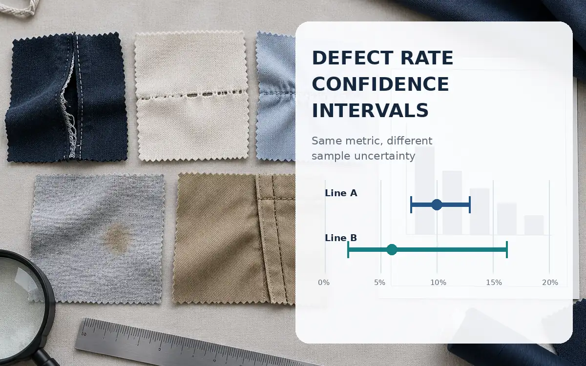
NIST's guidance on intervals for proportions describes Wilson and exact approaches. Under a binomial sampling model, a two-sided 95% Wilson interval for zero out of ten extends from zero to about 27.75%. That wide range shows how little ten clean observations can establish about a continuing process rate.

Use such intervals only with a suitable model. Records clustered by bundle or batch may not behave as independent trials. A full census of one finished lot also answers a different question from a sample used to infer a long-run rate.

The ApparelDiary Wilson interval guide explains the calculation in detail. For stratified comparisons, keep sample counts beside the rates and avoid precise rankings based on tiny cells.

Do not invent a rate for work a line has never done

Suppose a third line has no complex work in the period. Its complex-group rate is missing, not zero. A 50/50 standardized rate cannot be computed from observed group rates alone.

One option is to compare all three lines only on the group they share. Label that restricted scope. Another is to collect suitable evidence from a controlled trial of complex work. A model could estimate a missing rate, but the estimate must be labeled and checked.

Do not quietly drop the empty group for just one line while keeping the original weights for the others. That gives each line a different basis and restores the problem that standardization was meant to solve.

The same issue appears when styles differ greatly within a broad group. Check that “complex” means comparable work on both lines. Common labels are not enough if one line handles a different fabric, seam system, or inspection requirement.

Separate comparison from a claim about cause

The grouped example shows an association. It does not establish that moving an order to A would cause fewer faults. Line assignment may depend on skill, equipment, order risk, delivery pressure, or material quality. Some of those factors may remain unmeasured.

Choose grouping variables with process knowledge. Ask whether a field describes work assigned before the outcome or something changed by the line's own performance. Adjusting for a consequence of the process can obscure the effect being studied.

For example, do not compare lines only among garments sent to repair and then call the result overall quality. Entry into repair already depends on an observed problem. The selected subset can create a misleading relationship.

Use the analysis to design the next check. Comparable trials, matched work, and suitable statistical models can help answer a causal question. Their design needs more than a pivot table and a reversed ranking.

Read a cross-tabulation without changing its meaning

A cross-tabulation places categories in rows and columns. NIST's guide to classification tables shows how such tables organize relationships. For the main example, retain both affected and unaffected counts within each line and product group.

Be clear about the denominator of each percentage. “Complex work is 60% of A's inspected garments” describes A's mix. “A has a 6% affected-unit rate in complex work” describes an outcome within that group. Those percentages answer different questions.

A table containing only defects cannot recover the number of unaffected garments. It can show the composition of recorded faults, but it cannot establish an affected-unit rate. Add the inspection denominator from a compatible source and check the join.

Formal tests of association need their own assumptions. Sparse cells and linked observations can make a routine test misleading. Treat a statistically significant association as evidence of a pattern under the model, not proof of its practical importance or cause.

Build a repeatable calculation workflow

Begin with a dated copy of the eligible data. Apply the agreed first-pass and date filters. Check duplicate event identifiers, missing group codes, and impossible counts. Then group by line and product group.

For each group, sum the affected units and inspected units. Divide only when the denominator is greater than zero. Preserve an empty result for no inspected work rather than forcing it to zero.

Next, reconcile the grouped totals to the source log. Calculate each line's pooled rate from totals. Join the reference weights by exact group code, then multiply each valid group rate by its weight. Sum those products only when all required groups are represented.

Keep a small control table with the metric definition, period, source version, reference mix, exclusions, and reviewer. A later correction to one source record should refresh all affected views together.

Diagnose warning signs before the meeting

Report a useful next action

Give the production team a short explanation of the actual mix and observed group results. Show which difference deserves a closer look and which data limit prevents a firm conclusion. Name the next check and the work it should cover.

For the hypothetical case, the team might review complex work on B across more comparable orders. It could check material lots, method changes, and inspector agreement. Keep the question open until evidence supports an explanation.

Use a Pareto chart when the next task is to rank fault categories within a defined scope. Stratification has done a different job here: it made the between-line rate comparison interpretable.

Frequently asked questions

Should every dashboard use adjusted rates?

No. Actual counts and pooled rates answer important questions about real output. Add adjustment when a defined mix difference affects the comparison. Always retain the underlying groups and counts.

Can I use standard minutes as the weight?

Only for a measure whose question justifies that weighting. For an affected-garment proportion at a common product mix, the weights describe garment shares. Weighting by minutes creates a different index and needs its own label and interpretation.

Is a reversal proof that the adjusted result is correct?

It proves that aggregation matters in the dataset. Choosing the right comparison still needs process knowledge, valid measurement, and a clear question. Neither the pooled nor adjusted number answers every question.

How many groups should I use?

Use enough to represent the important differences in the work. Stop before the split creates mostly empty or tiny cells. Review the grouping with people who know the process and test its sensitivity.

Make the comparison explainable

Begin with a defined inspection event and a valid denominator. Split by relevant work conditions, show the rates within those groups, and inspect the weights behind the total. A common-mix rate can then support a fairer descriptive comparison. Keep its limits visible so the analysis leads to a well-chosen investigation, not an unsupported ranking.

References

ASQ. Stratification.

ASQ. Check sheet.

Teuscher, F. The quantification of Simpson's paradox and other contributions to contingency table theory. PLOS ONE, 2022.

CDC, National Center for Health Statistics. Standardization of rates, Statistical Notes No. 6, revised, 1995.

NIST/SEMATECH. Confidence intervals for a proportion.

NIST/SEMATECH. Comparing results classified by several categories.