Chiller Plant Efficiency for Textile Mills with COP and System Boundaries

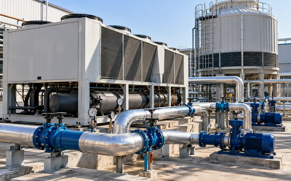
Measure cooling delivered and power used

A chiller can use less electricity because it is more efficient. It can also use less because the factory needs less cooling. Those are different results. To judge textile chiller plant efficiency, measure the cooling delivered and the power used to deliver it.

Start with a clear service requirement. A process may need water within a set temperature range. An air handler may need enough cooling to control room moisture. A lower plant meter reading is not a success if either service fails.

This guide covers the water side of cooling. It explains cooling load, coefficient of performance, system limits, and low chilled-water temperature difference. It also shows how pumps and towers can change the conclusion. Air distribution and room humidity need their own checks.

All examples below are hypothetical. The values show the method and its limits. They are not typical savings claims or performance targets for textile mills.

Draw the plant boundary first

List every item inside the energy measurement. Include each chiller, chilled-water pump, condenser-water pump, cooling-tower fan, and relevant control or standby load. Mark the meter serving each item. A shared feeder may cover more than the cooling plant.

Next, mark where cooling output is measured. At a chiller evaporator, the result describes heat removed from the water there. At the factory distribution header, it describes cooling delivered across that header. Pipe heat gains, pump heat, and storage can create a difference between the two.

Use one drawing for both sides of the ratio. AHRI's liquid-chiller guidance places the chiller within a larger system of pumps, controls, and heat rejection equipment. The whole system matters when a factory pays for delivered cooling.

Write the boundary beside every result. Two numbers called “plant COP” may include different pumps. A label alone does not make them comparable.

Calculate cooling from water flow

For a liquid stream with no phase change, the heat rate follows a basic energy balance:

Cooling rate = mass flow × specific heat × temperature difference.

In useful SI units:

Q = m × cp × ΔT.

Here Q is cooling in kW. Mass flow m is in kg/s. Specific heat cp is in kJ/(kg·K). The temperature difference ΔT is return temperature minus supply temperature, in kelvins. A temperature difference of 6°C has the same size as 6 K.

If the meter reports volume flow, convert it to mass flow:

Mass flow = volume flow in m³/h × density in kg/m³ ÷ 3,600.

Use fluid properties at the relevant conditions. Plain-water values are an approximation. A glycol mixture needs its own density and specific heat. Confirm the actual mixture instead of selecting a convenient water constant.

The DOE chiller evaluation protocol uses simultaneous flow and supply/return temperature measurements to establish cooling load. It distinguishes process cycles from seasonal HVAC loads. That distinction helps determine when and how long a textile plant should log data.

Do not substitute design flow for measured flow. A constant-speed pump does not prove constant flow. Valve positions, parallel pumps, and system resistance can change its operating point.

Work through one measured operating point

Assume a hypothetical water loop has these readings:

Mass flow = 150 × 998 ÷ 3,600 = 41.583 kg/s.

Temperature difference = 13 − 7 = 6 K.

Cooling rate = (150 × 998 ÷ 3,600) × 4.18 × 6 = 1,042.91 kW.

The result is thermal power, not electricity. A chiller moves heat, so its cooling output can be several times its electrical input.

Chiller COP = cooling output ÷ chiller electrical input.

Chiller COP = 1,042.91 ÷ 190 = 5.49.

COP is a ratio with matching power units. It is not a percentage efficiency like a motor's efficiency. A COP above one does not violate the energy balance; the machine transfers heat from the cold side to the hot side.

Record the operating conditions with this result. Include load, supply temperature, condenser conditions, active machines, and fluid. A COP without those details cannot support a fair comparison with a catalogue or another day.

Add auxiliaries before calling it plant efficiency

Suppose the same hypothetical plant also uses 25 kW for chilled-water pumps. Condenser-water pumps use 18 kW and tower fans use 12 kW. Assume all relevant loads are included and the cooling boundary remains unchanged.

Total plant power = 190 + 25 + 18 + 12 = 245 kW.

Plant COP = 1,042.91 ÷ 245 = 4.26.

The chiller COP was 5.49, but the plant COP is 4.26. Both are valid for their stated boundaries. Using the first figure to value whole-plant electricity would omit 55 kW at this operating point.

Check the boundary even when using an official worksheet. The North Carolina chiller fact sheet illustrates a calculation that omits chilled-water pump input. A factory-wide comparison may need that input included. This is why the equipment list matters more than the heading above the formula.

Avoid double counting packaged components. An air-cooled chiller's feeder may already include condenser fans. Adding their nameplate powers again would overstate input. Read the wiring and metering arrangement before summing loads.

Convert between COP and kW per ton

One refrigeration ton is about 3.51685 kW of cooling. It is a heat-rate unit. It does not describe the physical mass of a chiller or a tonne of textile output.

For the example:

Cooling tons = 1,042.91 ÷ 3.51685 = 296.55 refrigeration tons.

Plant kW per ton = 245 ÷ 296.55 = 0.826 kW/ton.

For matching boundaries, kW/ton = 3.51685 ÷ COP. Lower kW/ton is better. Higher COP is better. Both state the same relationship in different forms.

Do not mix rated tonnage with actual power. Dividing 245 kW by a 400-ton nameplate would give 0.613 kW/ton. That would be misleading if the plant were actually delivering only 296.55 tons. Use measured output for the operating result.

Keep “ton” and “tonne” clear in the report. A cooling-ton-hour is thermal energy. A tonne of finished fabric is production mass. A ratio using either needs its units written out.

Separate ratings from site performance

Standard ratings help buyers compare equipment under defined conditions. They do not reproduce every factory load, weather pattern, or control sequence.

AHRI 550/590 and 551/591 define rating methods for covered packages. Check the adopted edition and scope when requesting data. The public catalogue includes 2026 editions, so an old bid template should not silently define the current requirement.

Integrated part-load value, or IPLV, combines specified rating points. It is useful for its intended comparison. It is not a measured annual plant COP. A textile process that runs steadily through hot weather may have a different load and temperature pattern.

Ask suppliers for performance at the site's expected conditions. Include leaving chilled-water temperature, condenser conditions, fluid, flow, load, and power boundary. Request the operating limits as well as efficient points.

The DOE chiller purchasing guidance distinguishes equipment selected for full-load and part-load operation. Its procurement limits apply to its stated US federal context. Use the selection principle here without treating those limits as universal textile-factory rules.

Diagnose a low chilled-water temperature difference

Low delta T means the measured return-to-supply temperature difference is smaller than the expected value for that duty. It is a symptom. It does not name the cause.

At the same cooling load and fluid properties, halving ΔT doubles the required mass flow. For the earlier load, a change from 6 K to 3 K would require 300 m³/h instead of 150 m³/h. This follows directly from the heat balance.

That extra flow can use distribution capacity and affect staging. It may make the plant start another pump or chiller before cooling demand reaches the expected limit. The actual result depends on the piping and controls.

Start diagnosis at the sensors. Check their locations, calibration, and time alignment. Then inspect bypass paths and mixing. Compare coil branches at the same operating state. Look for valves that pass water when the load is low or the coil is off.

Also check whether coils can transfer the required heat. Airflow, fouling, valve control, and the required air condition can all matter. Do not assume every low-ΔT event means excessive water flow. At low load, the expected operating difference may also be lower than the design value.

Use branch evidence to locate the cause

Build a short branch log. Record flow, supply and return temperatures, valve command, fan state, and process condition. Read it alongside the main-header trend.

Treat each row as a test question. Do not order a valve replacement from the table alone. A control command is not proof of valve travel, and valve travel is not proof of flow.

After a correction, repeat the state that exposed the fault. Check useful cooling, not merely a warmer return. Restricting flow until ΔT rises may starve a coil and fail the process.

Check measurement error at small delta T

Temperature-difference error matters more when the true difference is small. Two accurate-looking temperature displays can still give a weak heat measurement.

Assume each hypothetical sensor has an error bound of ±0.1 K. The worst opposing errors create ±0.2 K in their difference. At a 6 K difference, that is 3.33%. At a 2 K difference, it is 10%.

Suppose the flow measurement also has a ±2% bound. Ignoring fluid-property error, the upper heat-rate bound at 6 K is:

1.02 × (6.2 ÷ 6) − 1 = 5.4%.

At 2 K, the corresponding upper bound is:

1.02 × (2.2 ÷ 2) − 1 = 12.2%.

These are conservative bound examples, not a formal uncertainty budget. A statistical method needs evidence about distributions and shared errors. Still, the calculation shows why a tiny apparent improvement may be unconvincing at low ΔT.

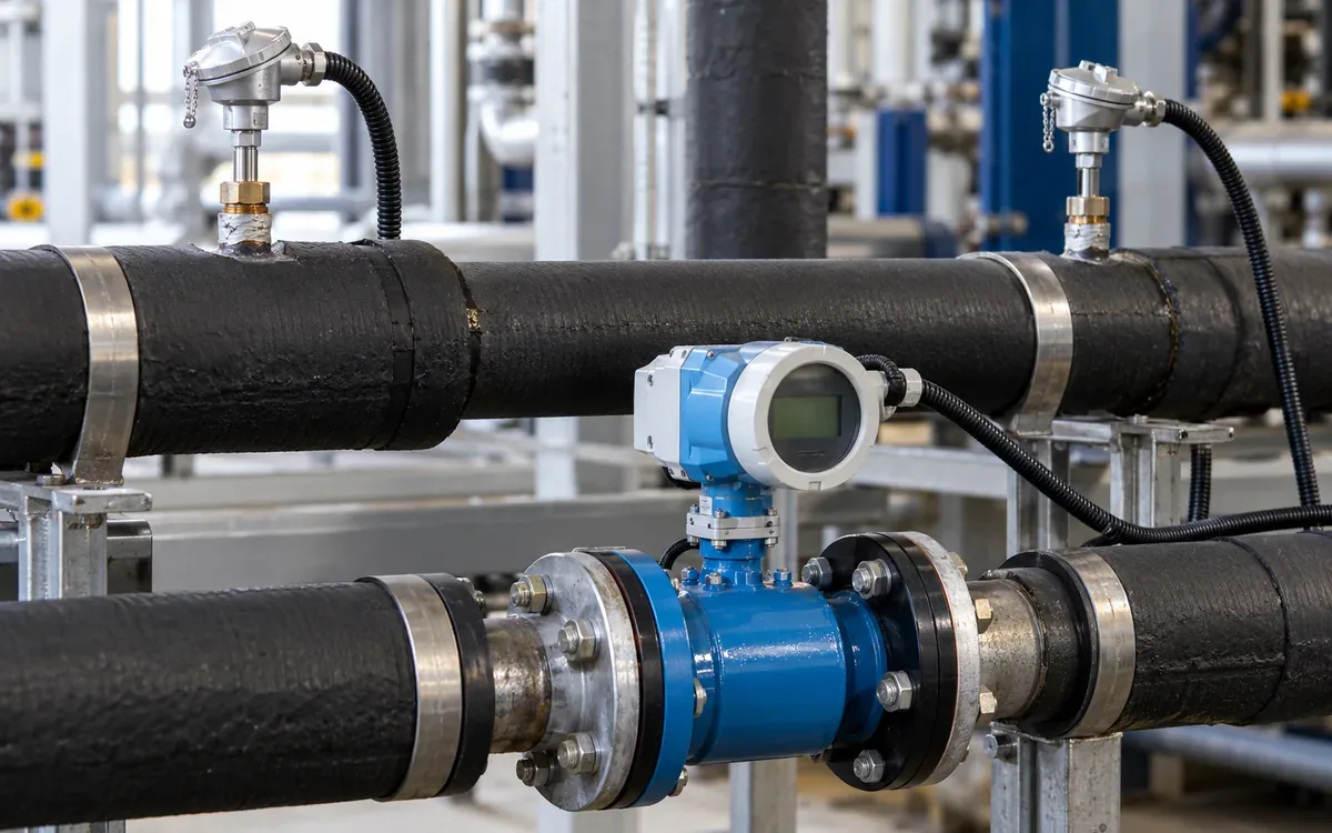
Use matched temperature sensors and suitable installation methods. Check paired readings under known equal conditions where practical. Confirm sensor immersion, contact, and insulation. For flow, verify pipe data and installation requirements. More decimal places on the display do not cure a poor measurement setup.

Optimize the tower and chiller together

Colder condenser water can reduce compressor work within the machine's limits. Producing that colder water can require more tower fan power. The best chiller point may therefore differ from the best plant point.

Trane's myPLV documentation describes models linking tower control, condenser conditions, and component energy. It also states model assumptions. Use such tools to compare defined cases, then check them against the actual plant.

Consider this hypothetical trial at equal delivered cooling:

Trial B saves 8 kW at the chiller but adds 14 kW at the tower. Plant input rises by 6 kW. Selecting the colder setting from the chiller reading alone would make this plant worse at that state.

Keep the manufacturer's operating limits in force. Review water treatment, tower condition, and stable control. Avoid a fixed promise that every degree of colder water creates the same percentage saving.

Review chilled-water temperature and pump control

A warmer chilled-water supply may reduce refrigeration lift. It may also reduce coil capacity or moisture removal. The allowed reset depends on the users and the operating state.

Define a trial range with the process and HVAC teams. Trend the most demanding users. Set stop rules before the test. Include humidity service where coils remove moisture. A room temperature target alone may miss that duty.

For pumps, review the pressure sensor location and the control target. A high fixed pressure can force valves to throttle. A lower target may save power, but it must still serve the critical path and meet chiller flow limits.

Do not promise an eightfold pump-power change merely because flow doubles or halves. Ideal affinity relationships require stated conditions. Real plants include static effects, changing efficiency, valve losses, and minimum flow. Measure the system result.

Use the factory utility load register when new equipment adds cooling demand. Record its required flow and temperature, not just its nameplate capacity. Update the hydraulic review and controls before connection.

Aggregate energy instead of averaging COP

An annual efficiency needs totals over the same time period. A simple average of spot COP values usually gives the wrong weight to each condition.

In a hypothetical day, the plant delivers 1,000 kW of cooling for two hours at 200 kW input. It then delivers 400 kW for six hours at 100 kW input.

First period cooling = 1,000 × 2 = 2,000 kWh thermal.

Second period cooling = 400 × 6 = 2,400 kWh thermal.

Total electrical energy = 200 × 2 + 100 × 6 = 1,000 kWh.

Period COP = (2,000 + 2,400) ÷ 1,000 = 4.4.

The spot COP values are 5 and 4. Their simple average is 4.5, which is not the period result. Integrate cooling and electrical energy, then divide the totals.

Include relevant standby energy in the stated annual boundary. If the plant uses electricity while delivering no cooling, a spot COP is not useful for that interval. The energy still belongs in the annual denominator when the boundary includes it.

Estimate savings by operating state

Compare old and proposed performance at equal service. Use credible hours for each state. Keep the load and weather assumptions visible.

The following hypothetical comparison uses whole-plant COP values, including the stated pumps and towers:

For each row, electricity equals cooling load × hours ÷ COP. The estimated total reduction is about 82,828 kWh/year. These assumed COP values need measurement or supported performance data in a real proposal.

Do not add a separate pump saving if the proposed plant COP already includes it. Add any excluded load only with a clear boundary adjustment. Test a less favourable duty schedule before accepting the investment case.

Price energy using the avoidable tariff component. Assess demand-charge effects separately. For broader financial treatment, use ApparelDiary's guide to discounting factory cash flows.

Compare staging options at the same load

More machines running does not always mean more energy. Nor does loading one machine as far as possible always give the best result. The answer depends on the equipment and its auxiliary loads.

Imagine a hypothetical 700 kW cooling demand. One available chiller arrangement uses 150 kW at the package and 45 kW in auxiliaries. Total input is 195 kW. A two-chiller arrangement uses 138 kW across the packages but 68 kW in auxiliaries. Its total is 206 kW.

The two packages are more efficient at this assumed point, yet the plant uses 11 kW more. The added pumps and towers reverse the choice. A different load or different equipment could reverse it again.

Build a staging map from measured or supported plant data. Include minimum and maximum flows, stable load ranges, start limits, and required reserve. Set a reasonable delay or dead band so small load changes do not trigger repeated switching.

Test changeover as well as steady running. Check supply temperature, pressure, and critical users while another chiller starts or stops. An efficient steady point is of little value if the transition repeatedly disrupts the process.

Keep the approved map with the control sequence. Review it after equipment replacement or a major process change. A sequence designed for the old machines may no longer suit the new plant.

Place meters where the balance can close

Choose the flow and temperature points as a matched set. A flow meter on one branch and temperatures on a mixed header do not describe one water stream. Draw the pipe path between all three points.

Identify bypasses, storage tanks, and other connections between the meters. These can change the mass or heat balance. If storage is charging, evaporator output can exceed cooling sent to users. During discharge, the reverse can occur. Record storage state before comparing those boundaries.

Check time intervals too. A one-minute temperature average paired with an hourly flow total can hide a short process peak. Use suitable coincident data to calculate interval heat, then sum it. Multiplying unrelated averages can create a false result when flow and temperature difference vary together.

For a temporary meter, record the exact installation and settings. Keep the pipe size, wall data, fluid choice, and sensor position with the results. That makes a later repeat survey comparable and helps explain a sudden change after the meter is moved.

Keep the operating record useful

Create one record for each stable test period. Include cooling output, all included electrical loads, active equipment, water temperatures, flow, outdoor condition, and production state. Record alarms and manual overrides.

Flag bad data before calculation. A negative cooling value may reveal swapped sensors, reverse flow, a shutdown transition, or a real heat-flow change. Do not silently replace it with zero. Investigate and document the rule used to exclude it.

Keep starts and transitions for service analysis even when they are excluded from a stable-point comparison. A plant that cycles often may look good in selected snapshots while wasting energy over the full day.

Assign each recommended change an owner and an acceptance test. State the useful cooling that must remain available. Record both successful and failed trials so later teams know the tested limits.

Frequently asked questions

What is a good COP for a textile chiller plant?

There is no useful universal answer without a boundary and duty. Cooling temperature, heat-rejection conditions, load, fluid, and auxiliaries all affect the result. Compare with supported performance for the same service.

Does low delta T prove that the chiller is inefficient?

No. It describes the water temperature difference. Check sensors, flow, mixing, coil duty, and controls. Assess chiller and plant efficiency with measured cooling and input power.

Can the chiller screen replace independent metering?

It can provide useful data if its points and calculations are verified. Check the sensor basis and electrical boundary. Do not assume every displayed load or efficiency value is a direct measurement.

Should a new chiller be selected only by IPLV?

Use standardized ratings for comparison, then assess the site's duty. Request suitable full-load and part-load data. Include auxiliaries, operating limits, and the required service in the final choice.

Conclusion

Chiller plant efficiency is a relationship between useful cooling and all included input energy. Define that relationship before collecting readings. Measure flow and paired temperatures, include auxiliaries, and compare equal service.

Use low delta T and high component power as clues. Confirm their causes through branch data and controlled trials. A sound improvement reduces total plant energy while preserving the cooling conditions the factory needs.

References

DOE/NREL, Chapter 14: Chiller Evaluation Protocol, 2017.

AHRI, Liquid Chillers.

AHRI, Standards 550/590 and 551/591 catalogue and scope.

US Department of Energy, Purchasing Energy-Efficient Electric Chillers.

North Carolina, Energy Saving Fact Sheet: Chillers.

Trane, myPLV tool assumptions and explanations.