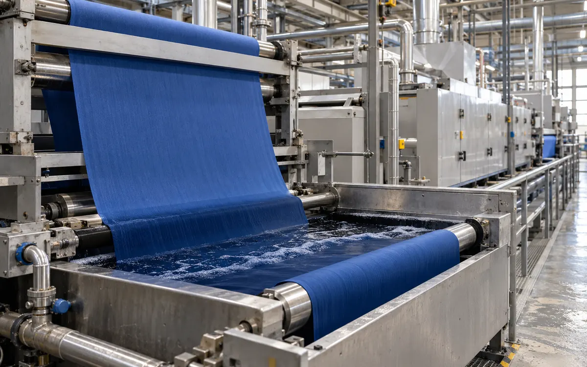
Tailing and Listing in Continuous Fabric Dyeing

Mark the cloth in two directions before changing the recipe

Tailing and listing describe where shade changes appear in a fabric run. Tailing is variation along the length. Listing is variation across the width. It may appear as a side-to-centre or side-to-side shade difference. A roll can contain both patterns.

The useful first step is to preserve that pattern. Mark each sample's length and width position. Label the face and running direction. Link it to the process conditions that this cloth experienced.

A darker end alone does not prove that the dye feed was too strong. An edge mismatch alone does not prove that the padder needs more pressure. Preparation, application, drying, fixation, and washing can each affect the final shade.

This article sets out a practical investigation for open-width continuous dyeing. The calculations use teaching examples with stated assumptions. They help diagnose faults. They do not set machine limits or approve recipe changes.

Build a two-direction shade map

Collect matched width positions at several known length positions. Choose locations and sampling frequency to suit the process. Consider the buyer's requirements and the observed fault too.

Keep left and right defined from one stated viewing direction. One person may stand at the entrance and another at the exit. They can then mean different edges by “left”.

Record an agreed colour measure on the map. Add visual observations alongside it. Do not reduce the whole roll to one average before looking at its structure.

Consider these hypothetical CIELAB lightness readings, measured under the same conditions:

Length position	Left L*	Centre L*	Right L*	Row mean
100 m	40.2	40.0	39.8	40.0
1,100 m	39.8	39.6	39.4	39.6
2,100 m	39.4	39.2	39.0	39.2

The row mean falls by 0.8 lightness unit through the sampled length. At every row, the right side is 0.4 unit below the left. This example shows two patterns. There is lengthwise drift and a stable difference across the width.

The map does not establish the cause or the pass decision. L* alone omits hue and chroma. One pooled number would hide those patterns. The map keeps useful evidence for diagnosis.

Add events to the same map

Mark seams between input rolls, starts, stops, tank changes, speed changes, and adjustments. Include any sample gaps.

A shade boundary may follow a roll seam. Check the input difference and how the process handled that join. A boundary may instead follow a feed-tank change after the expected delay. In that case, compare the two liquor preparations.

The relationship is evidence for the next check. It is not proof of causation. More than one event may occur close together.

Check that the colour comparison is valid

Hot, damp cloth may look different from a dry lab reference. That difference need not be a lasting dyeing fault.

Datacolor's guidance on accurate colour data describes the effects of temperature and moisture on measurement. Use the agreed specimen condition before making a release comparison.

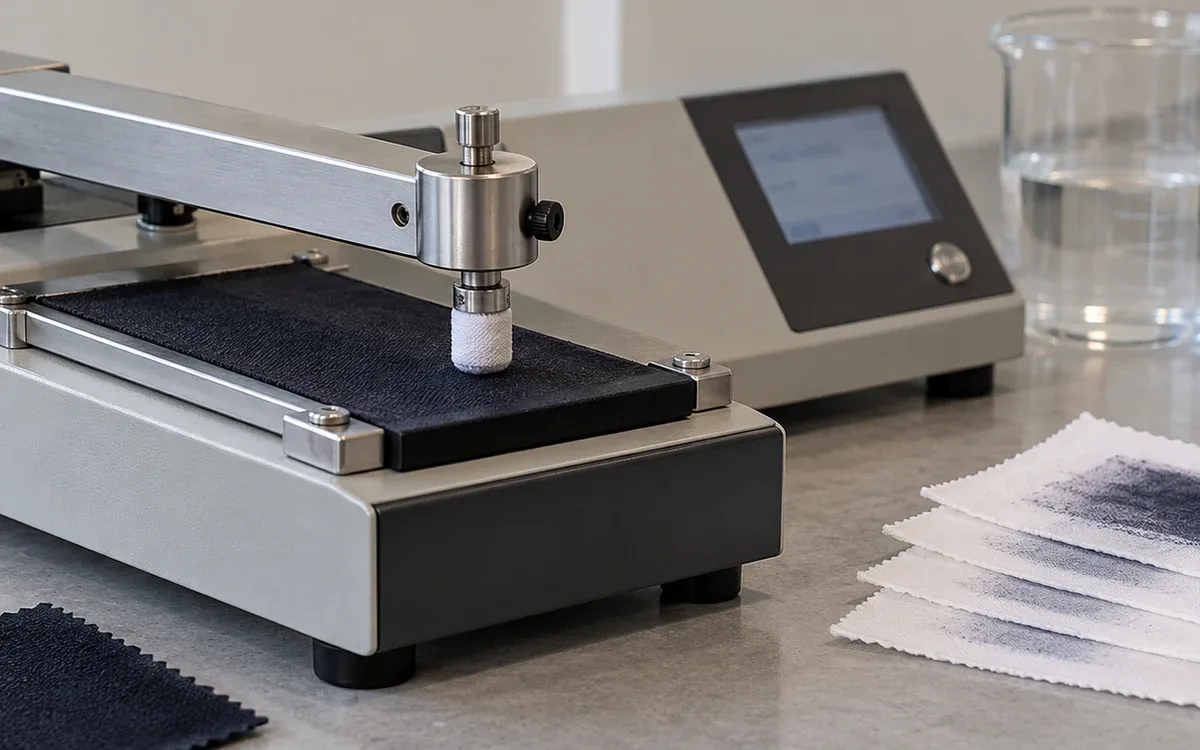
Record the instrument setup, colour-difference method, and sample presentation. ISO 105-J01 gives a framework for instrumental surface-colour measurement. Its public scope does not contain the full procedure.

Keep the investigation focused on process origin. ApparelDiary's fabric shade segregation guide explains how to keep approved shade groups through cutting. Separating a roll can control its use. It does not correct the dyeing process.

Trace the fabric through the actual range

Draw the process path used for the order. Identify application, drying, fixation, washing, and final drying stages. Include the sample points and the distance between them.

Continuous and semi-continuous routes have different steps. See the European Commission's textile reference document in section 2.7.2.2. It describes continuous application. In some routes, later fixation or washing occurs in separate batches.

Use the actual route when connecting a defect to an event. Pad-batch uses a dwell stage. Its time record differs from that of an uninterrupted pad-steam range.

Do not assume that a reading at the exit describes the current condition at the padder. The cloth between the two points carries an earlier process history.

Calculate the transport delay

Suppose the fabric path from the padder to an inspection point is 240 metres. At a steady 30 metres per minute:

Transport delay = path length ÷ line speed

240 ÷ 30 = 8 minutes

Suppose the defect appears at 14:22. Under these assumptions, that cloth passed the padder at about 14:14. A feed change at 14:18 cannot explain its padder exposure.

Now let the first 120 metres travel at 30 m/min. Let the next 120 metres travel at 20 m/min. The delay is:

120 ÷ 30 + 120 ÷ 20 = 4 + 6 = 10 minutes

Using the normal-speed eight-minute value would connect the sample to the wrong event.

For stops and changing speeds, use encoder length and time records where available. Keep the clocks on the range, dosing system, and laboratory aligned.

Treat a stop as several different exposures

When the range stops, cloth occupies several zones. Some is near the padder, some is under heat, and some is in washing. These sections experience different conditions. A single label saying “stop mark” can hide that distinction.

Use the threaded path to identify which fabric occupied each section. Record the stop time, duration, and restart sequence. Add any automatic machine response. Account for movement, then compare later defect positions with those locations.

The first cloth after restart may look acceptable. It may have been downstream of the disturbed stage during the stop. Its appearance cannot prove that every upstream stage is stable again.

Keep samples from the transition until the affected interval is understood. If there are two separate bands, check whether they correspond to two process zones. The bands may follow the same alarm. That does not prove one cause for both.

This event record also helps assess a proposed recovery. Some cloth may have had unusual heat exposure. Other cloth may only have had a brief change in liquor application. These sections may need different performance checks. Judge each by its exposure and test evidence. Do not assume all metres made around the stop are the same.

Confirm pickup on the fabric

Wet pickup expresses retained liquor relative to the stated dry fabric mass. For a defined weighing procedure:

Pickup (%) = (wet mass − dry mass) ÷ dry mass × 100

Control evaporation and sample handling during the procedure. Define the dry-mass basis. If an input specimen already holds water, account for it in the method.

Consider three hypothetical dry specimens, each weighing 20.0 g. After the same padding operation, their measured masses are 34.0, 34.0, and 36.0 g.

The pickups are 70%, 70%, and 80%. The third location retains 14.3% more liquor per unit dry mass than the first:

(80 − 70) ÷ 70 × 100 = 14.3%

At the same uniform liquor composition, that changes the amount of dye liquor carried forward. Final colour may not change in the same proportion. Fixation, migration, washing, and optical response also affect it.

A pressure setting is not a pickup result

The padder setting is an input to the process. Pickup is an observed fabric response. Keep both in the investigation.

Kusters Calico describes two separate controls. See the line-force and bending-control functions in its dyeing padder information. One pressure display alone cannot describe squeezing across the full width.

Follow the machine supplier's inspection procedure. Check roll condition, alignment, and the loading system. Review relevant maintenance records. Use approved tests to assess evenness.

Never reach into a running nip. Do not change protective systems to take a sample. Use the equipment's approved safe arrangements for sampling and maintenance.

Convert fabric throughput into expected liquor demand

Start a feed calculation with the fabric mass passing the padder. Speed alone is not enough.

For the following dry-entry example:

Dry fabric rate = mass per area × working width × speed

Assume 220 g/m² fabric, a working width of 1.60 m, and a speed of 35 m/min.

Convert 220 g/m² to 0.220 kg/m²:

Dry fabric rate = 0.220 × 1.60 × 35 = 12.32 kg/min

At 70% net pickup:

Liquor carried out = 12.32 × 0.70 = 8.624 kg/min

Assume a liquor density of 1.00 kg/L. The corresponding volume is 8.624 L/min. For a real calculation, use the correct density. Use a pickup basis proved valid for the route.

This is a simplified steady-state estimate. It excludes evaporation, leaks, overflow, and other streams. It describes the net liquor leaving with initially dry fabric.

A heavier fabric changes the feed requirement

At the same width, speed, and pickup, 260 g/m² fabric gives:

0.260 × 1.60 × 35 × 0.70 = 10.192 kg/min

That is 18.2% more than the first fabric's liquor carry-out. Leaving the feed at its previous value would not preserve the simple balance.

Use fabric mass measured at the relevant stage. A greige value can differ from the prepared fabric entering the dye range.

For wet-entry processing, account for incoming liquid and liquor exchange. The dry-entry formula does not directly fit wet entry. Adapt it before calculating chemical replenishment.

Separate level control from composition control

A trough can stay at the correct level while its dye composition changes. Level control replaces volume. It does not independently verify each dye component or auxiliary.

Check the delivered feed, including pump performance and actual mixing. A controller may command eight litres per minute. That does not prove eight litres reached the trough.

Where streams mix just before application, verify their ratio and timing. A correct combined flow can still contain an incorrect dye-to-auxiliary ratio.

Benninger identifies its two-roll DyePad within its continuous and cold pad-batch systems. Equipment capability helps establish control options. The mill must still verify the composition and delivery of the liquor it uses.

Reconcile a short time interval

Take an example ten-minute interval. The trough starts and ends with the same measured inventory. The feed meter records 90 litres. Estimated fabric carry-out is 86 litres.

The unexplained difference is four litres:

90 − 86 = 4 litres

Check for other withdrawals, additions, and evaporation. Look for measurement error or changes hidden by the level reading. Do not call the difference a leak without evidence.

Short balances are useful when the assumptions can be checked. A brief feed break may cause a visible shade band. A daily total can hide that break.

Understand trough turnover before making another correction

A change in feed composition takes time to move through a mixed inventory. The first cloth after an adjustment may still carry mostly the earlier liquor.

A simple ideal mixing model gives a useful scale for that delay:

Turnover time = effective mixed volume ÷ throughflow

Take an example well-mixed system containing 60 litres. Its throughflow stays at 10 L/min. Turnover time is six minutes.

Suppose feed concentration suddenly changes to a new value. After one turnover, about 37% of the initial concentration difference remains. After three turnovers, about 5% remains. These figures come from the ideal model.

The relationship is:

Remaining fraction of the initial difference = exp(−time ÷ turnover time)

Here “exp” is the exponential function. It describes gradual replacement in a perfectly mixed system.

At 30 m/min, one turnover covers 180 metres of fabric. Three turnovers cover 540 metres.

Use the model as a question, not a machine promise

A real system includes pipes and may recirculate liquor. Mixing may be imperfect. Chemical reaction and selective dye uptake can occur. These features can change the response from the ideal model.

The calculation explains why repeated quick corrections can create further shade swings. The first change may not yet have reached inspection. A second change would then be based on old information.

Run an approved trial to find the actual response. Use the normal process measurements. Account for both liquor response and fabric transport delay.

Do not introduce an unapproved tracer or chemical solely to make the response easier to see.

Consider dye compatibility and selective uptake

Each dye in a mixture may leave the padding liquor at a different rate. The bath can change hue even while its total volume stays constant.

The European Commission's textile reference discusses low-affinity dye selection. This can reduce unwanted exhaustion from a padding bath. Ask the supplier to help select dyes that work well together.

Use the complete dye system and application conditions in the trial. DyStar's Cadira reactive/disperse continuous process uses selected dyes and a defined process package. It is one example of this approach. It does not approve untested substitutions in another recipe.

When a drift changes hue, examine the component balance as well as overall depth. Adding more of the whole mixture may deepen the cloth. The wrong hue relationship can remain.

Use a lab trial to test the suspected dye behaviour. Keep its conditions relevant to the production route.

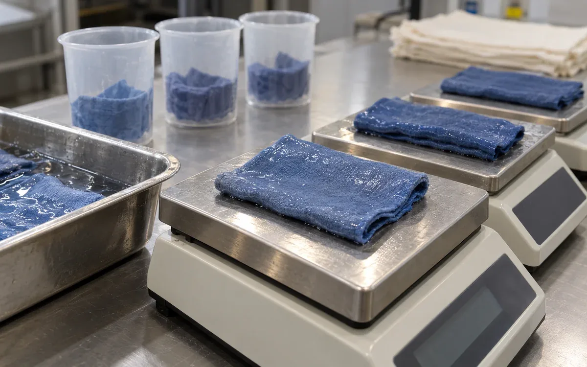
Tailing and Listing in Continuous Fabric Dyeing — process illustration

Look for where the difference first appears

A finished shade defect can have an upstream cause. Plan the investigation and sample stages. Take labelled samples where safe access and the method allow it.

Pickup may vary across the width just after padding. If so, check application and input fabric. Pickup may instead be even, with a colour pattern appearing after drying. Then check drying and migration before changing the padder.

If the pattern appears after washing, compare washing conditions and the state of the dye before that stage.

Stage comparisons must use a suitable assessment basis. A wet intermediate sample has not reached the same state as a dried, washed sample. Keep that difference clear in the comparison.

First clear evidence of variation	Main area to investigate
Prepared undyed fabric differs	Check input construction and preparation history.
Retained liquor differs after padding	Check application, fabric wetting, and squeezing.
Pattern develops during drying	Check moisture removal and airflow. Review temperature and dye movement.
Pattern develops during fixation	Check actual exposure and the chosen dye system.
Difference changes during washing	Check whether washing is even. Check removal of unfixed material.
Difference appears only after final finishing	Check finish application, drying, and appearance effects.

Examine drying and fixation across the width

The chamber display measures air temperature. It does not prove the same drying and fixation history across the fabric.

Monforts describes several controls in its continuous dyeing ranges. These include air control, temperature management, and fabric guidance. Examine them when a fault develops after application.

Check the actual route's required temperature, moisture, and dwell conditions. Do not copy one thermosol or reactive-fixation setting into another system.

A speed change also changes residence time. Take a heated path of 90 metres. At 30 m/min, residence time is three minutes. At 36 m/min, it is 2.5 minutes. That is a 16.7% reduction in nominal time.

The colour response need not change by the same percentage. Use the calculation to identify the exposure change that the trial must assess.

Measure the relevant moisture condition

Mahlo's process-control documentation describes several separate measurements. These include fabric moisture and surface temperature. Others measure dwell time and exhaust-air moisture.

Select the quantity that answers the fault question. Exhaust-air humidity cannot replace a fabric-moisture profile when the issue is a wetter edge.

Check the sensor's calibration and suitability for the material and process. An unsuitable measurement can still produce a detailed trend. More data points do not make it reliable.

Record sensor positions and scan timing with the data. These help explain the pattern across the width.

Include washing in the diagnosis

Continuous dyeing is not complete when colour first develops. Washing can change the shade and its uniformity by removing material from the cloth.

Check water flow, temperature, fabric contact, squeezing, and any specified wash chemistry. Keep conditions linked to the same fabric section used in the shade map.

A wash disturbance may follow an earlier padding fault. The finished pattern can then combine two effects. Preserve the sequence. Do not force every observation into one cause.

A lab wash may change the affected specimen. Compare it with an acceptable specimen washed in the same way. A change in both samples may be normal wash behaviour. A different response may help narrow the investigation.

Do not approve production recovery from colour alone. Retest the performance properties required for the product after the proposed route.

Use controlled trials to separate fabric and range effects

Take matched pieces from the affected and acceptable input positions. Process them under one controlled laboratory route where that comparison is meaningful.

If they still differ, examine the input or its preparation. If they converge, investigate what differed in production. Lab and production equipment may still treat the same fabric differently. Interpret this as evidence. It is not a final verdict.

For a suspected padder problem, compare measurements before and after a documented maintenance correction. Keep fabric, liquor, and other conditions stable enough to understand the result.

For a feed problem, reconcile the actual tank preparations and pump delivery before making another shade correction.

Change one defined factor at a time where possible. Several changes may be needed together. Record them as a package. Do not claim that one part alone caused the improvement.

Contain the affected fabric using measured boundaries

Mark the last confirmed acceptable section, the suspect interval, and the next confirmed acceptable section. Keep unsampled material visible as an evidence gap.

A sample at 1,000 metres may pass while one at 1,500 metres fails. This does not locate the exact start of the fault. More checks may narrow that boundary.

Preserve the physical identity of held sections when rolls are rewound, cut, or moved. The process team needs this link to investigate. Quality staff need it to control release.

Use the buyer's agreed shade and performance rules for disposition. A machine adjustment that improves later cloth does not automatically release fabric made earlier.

Prevent recurrence with a compact control record

Start the record with fabric identity, working width, and mass. Add pickup, actual feed, trough conditions, and line speed. Include key downstream measurements.

Keep measured values distinct from setpoints. Retain event times and sample positions in the same reference system.

Review startups, roll changes, tank transitions, and stops separately from steady running. A route may be stable in the middle of a long run. Each changeover can still be unreliable.

After a correction, compare the next relevant runs with the same measurements. Look for both reduced variation and fewer unexplained adjustments. A lower defect count may look promising. Check whether sampling was reduced at the same time.

Frequently asked questions

Can tailing and listing occur together?

Yes. A run may drift along its length while keeping a side-to-centre difference. A two-direction map helps separate the patterns.

Does constant trough level prevent tailing?

It helps control inventory, but it does not prove stable composition. Check feed ratios, dye uptake, mixing, and actual delivery.

Will higher padder pressure always improve listing?

No. The required setting depends on the equipment and fabric. Measure pickup and assess the across-width system before changing pressure.

Is the first sample after an adjustment enough?

Usually it cannot describe the full response. Account for mixed-liquor turnover, fabric travel, fixation, washing, and the agreed sample condition.

Can an online colour reading replace final approval?

Only within a validated control and acceptance system. Online data can give early warnings. Final release must follow the required stage, conditions, and buyer rules.

Correct the source of the shade pattern

To control tailing and listing, link the fabric map to timed process records. Pickup and feed calculations explain the material moving through the range. Stage comparisons show where the visible difference develops.

When those records agree, the next trial becomes more focused. The mill can then correct the process that caused the shade variation. Verify the result on the cloth the customer will receive.