Pump System Optimisation in Textile Mills with Curves and Power Checks

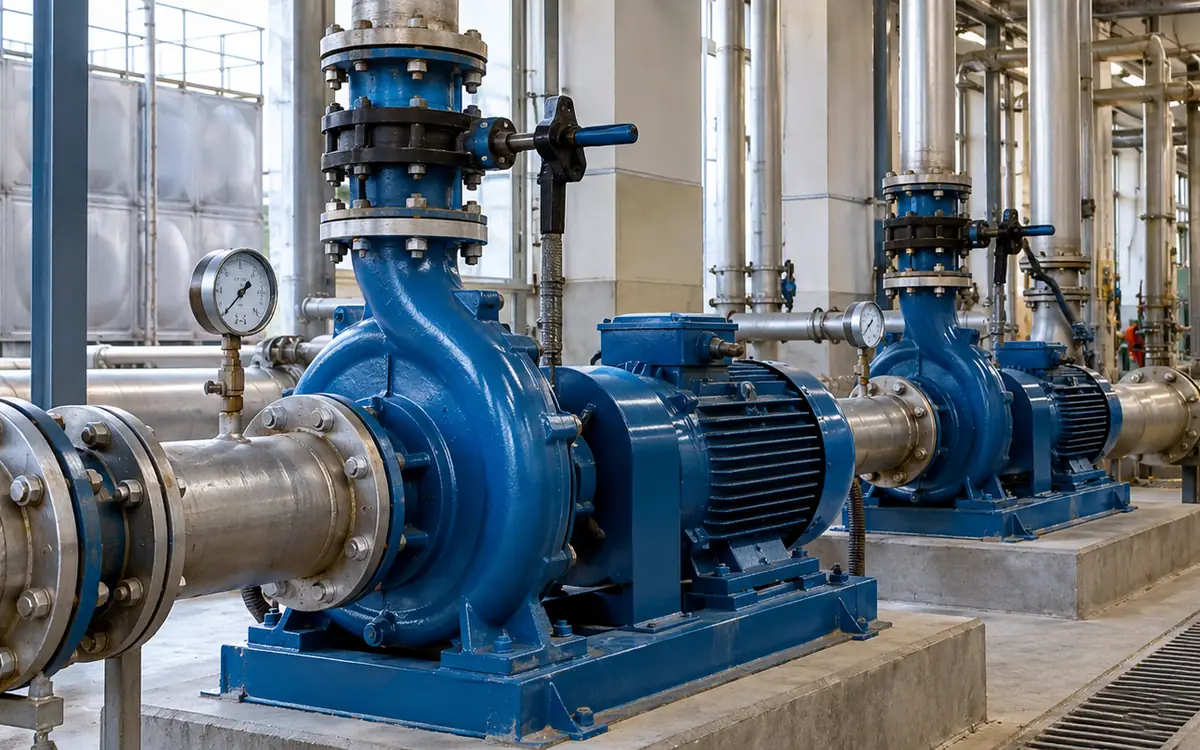
Start with the service that the water must provide

A pump can run smoothly and still use too much energy for its job. It may supply more head than the process needs. A valve may remove that extra head. A bypass may send part of the flow back to the tank.

The useful target is the required service: the right flow, pressure and timing at the user. Measure that need before choosing a smaller pump or a variable frequency drive, often called a VFD.

This guide concerns existing centrifugal pump systems in textile utilities. It covers water transfer, cooling and similar liquid duties. Special process pumps need their own limits. Fire-protection pumps and other safety systems must remain under their specific design and operating rules.

All numerical cases are hypothetical. The curves and efficiency values are teaching inputs. Use verified maker data and site measurements for a real change.

Set a boundary that includes the whole duty

Draw the source, pump, pipes, valves and receiver. Mark branches, bypasses, filters and heat exchangers. Note whether the flow transfers water to another level or circulates around a closed route.

Write the minimum service needed at the user. Include flow, pressure, temperature and any allowed change over time. A process may need a minimum velocity or cooling rate even when production is low.

Identify when the duty exists. A transfer pump may move a fixed daily volume. A cooling pump may need continuous flow during a process. The same speed change has different energy effects in those two cases.

Use the factory utility load register to confirm the connected service needs. Then measure the actual duty. A nameplate or purchase estimate is useful background, but it is not proof of current demand.

Separate static head from flow-dependent loss

Static head comes from level or pressure differences that exist apart from flow. A higher receiving tank creates a lift. A pressurised receiver can create another fixed requirement.

Friction head is the loss as liquid passes through pipes and equipment. In a common turbulent-flow model, it rises roughly with the square of flow. The coefficient depends on the route and its condition.

A simple system curve is:

H_system = H_static + K × Q².

Define the units used for Q before finding K. A coefficient fitted with m³/h cannot be reused with m³/s without conversion.

The joint DOE, Hydraulic Institute and Europump guide explains why the static-to-friction split matters. It changes how flow and efficiency respond to speed.

In a closed circulation loop, height gained on one part may be recovered elsewhere. Do not add the building height as a permanent pump lift without tracing the full hydraulic path. The actual boundary decides which level terms remain.

Read the operating point from both curves

A centrifugal pump curve shows the head the pump develops at each flow. A system curve shows the head the route needs at each flow. Their intersection defines a possible steady operating point.

The Hydraulic Institute's curve guide explains this interaction. It also shows how throttling, speed and impeller changes move the operating point.

A curve must match the installed speed and impeller diameter. Confirm the pump model and whether parts have changed. A curve for the largest available impeller may not describe the machine in the plant.

Also read the efficiency and power curves. Check the maker's preferred and allowable operating regions. The best efficiency point is useful, but the whole required range must be acceptable.

Do not infer pump wear from one low-flow reading. A partly closed valve, a changed tank level or a blocked filter can move the system curve. Test the system before deciding that the pump itself needs replacement.

Measure head correctly

Pump head includes more than a discharge gauge reading. Across suitable inlet and outlet measurement points, the steady total-head rise is:

H = (p_out − p_in) ÷ (ρ × g) + (v_out² − v_in²) ÷ (2 × g) + (z_out − z_in).

Pressure p is in pascals, density ρ in kg/m³, velocity v in m/s and elevation z in metres. Use g = 9.81 m/s² for the example calculations.

Where tap elevations and pipe velocities are effectively equal, the last two differences may be small. State that assumption instead of dropping the terms without explanation.

Use pressure readings on the same basis. A differential between two gauge readings is valid when their reference is the same. Record where the taps sit relative to the pump and any nearby loss.

The ASHRAE centrifugal-pump chapter provides the pump-performance framework. A field test still needs suitable instruments and a method that fits the pipe layout.

Make flow measurement fit the actual pipe

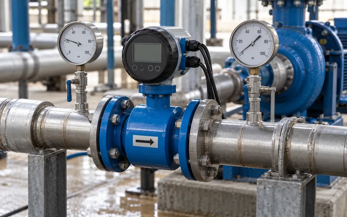
Check the pipe size, material, wall and lining before installing a temporary meter. Confirm that the pipe is full at the measurement point. Use the meter maker's guidance for straight lengths and nearby fittings. A convenient spot beside an elbow may give a poor basis for the whole project.

The liquid also matters. A meter suited to clean water may need a different setup for a stream with bubbles or solids. Choose the method for the actual fluid and duty. Keep its stated range and uncertainty in the test record.

For a steady transfer, a tank-level change over a known time may provide an independent check. It needs a valid tank-volume relation and a record of other inflows or outflows. If another pump is filling the same tank, the level change alone does not equal the tested pump's delivery.

Measure bypass and useful flow separately when they differ. A pump discharge meter might count water that never reaches the process. Mark the meter's position on the system drawing so the next reviewer understands what its total includes.

Synchronise flow, pressure and power readings. A flow taken during filling and a power reading taken during recirculation cannot form one efficiency point. Log the operating state beside each set, even when the measurement period is short.

Distinguish pump efficiency from electrical efficiency

Hydraulic power is the rate of energy added to the liquid:

P_hydraulic = ρ × g × Q × H ÷ 1,000.

With Q in m³/s, the result is kW. Pump efficiency compares this hydraulic power with shaft input. Electrical input also includes motor and drive losses.

For a drive-fed pump, a simple model is:

P_electric = P_hydraulic ÷ (η_pump × η_motor × η_drive).

Use efficiencies as fractions. Do not divide by 68 when the pump efficiency is 68%; use 0.68.

The DOE pumping-efficiency guide also stresses required head and flow. Unnecessary bypass flow and excess head do not become useful service merely because the pump produces them efficiently.

For a separate arithmetic check, assume water density 998 kg/m³, flow 90 m³/h and head 32 m. Hydraulic power is about 7.83 kW. With pump, motor and drive efficiencies of 0.68, 0.92 and 0.97, electrical input is about 12.91 kW.

That is a model result, not a motor nameplate rating. Measure real electrical power with suitable equipment when checking an installed system.

Work through a simple pump and system model

Consider these hypothetical curves, with Q in m³/h and H in metres:

H_system = 12 + 0.0025 × Q².

H_pump = 44 − 0.0015 × Q².

At the open-route operating point, set them equal. This gives 32 = 0.004 × Q², so Q is about 89.44 m³/h. The head is 32 m.

Suppose the process needs only 80 m³/h. The base system needs 12 + 0.0025 × 80² = 28 m. At the same flow, the full-speed pump produces 44 − 0.0015 × 80² = 34.4 m.

A discharge control valve can add 6.4 m of head loss and hold the flow at 80 m³/h. That achieves flow control, but the pump still supplies the extra head lost at the valve.

This calculation makes the opportunity specific. The issue is 6.4 m of excess head at one stated duty. It is not proof that every control valve should be removed or that the whole motor input is avoidable.

Compare throttling and speed at equal flow

For this ideal pump model, let n be the new speed divided by original speed. Applying similarity to the whole curve gives:

H_new(Q) = 44 × n² − 0.0015 × Q².

To provide 28 m at 80 m³/h, solve 28 = 44 × n² − 9.6. The speed ratio is about 0.9244. This model therefore needs about 92.4% of the original speed at that duty.

Use actual efficiency data for each point. In this example, assume the full-speed pump is 68% efficient and its motor is 92%. Electrical input is about 11.96 kW.

Assume the reduced-speed pump is 70% efficient, the motor remains 92% and the added drive is 97%. Electrical input is about 9.75 kW. The model saving is about 2.21 kW at equal useful flow and base-system head.

These efficiencies are hypothetical and must not be treated as generic performance. They show why a complete comparison includes pump, motor and drive. Omitting the drive loss or assuming the pump efficiency never changes can overstate the result.

Know where the cube law stops being enough

At similar pump operating points and roughly constant efficiency, flow scales with speed, head with speed squared and shaft power with speed cubed. These are the familiar affinity relationships.

They describe pump behaviour under their assumptions. They do not say that every installed system uses the cube of its original electrical power after a speed change.

The system in the example has 12 m of static head. That part does not shrink with flow. As speed falls, the new intersection may move across the pump's efficiency map. Motor and drive efficiency may also change.

The Hydraulic Institute's variable-speed discussion shows why the system curve and operating range need review. At too low a speed, a pump may not overcome the required head at all.

Use affinity laws to form a screening model. Then use rated curves and system intersections across the required range. Check minimum flow, suction conditions, motor cooling and other maker limits before choosing a speed range.

Consider impeller trimming for a lasting duty change

If the required duty is nearly constant, a suitable smaller impeller may be worth comparing with a drive. It changes the pump curve without adding continuous speed control.

The DOE impeller-trimming guide calls for maker curves and limits. A large trim can change clearances and efficiency. Suction-head requirements may also change.

Ask the maker for a rated trimmed curve at the required flow. Include power, efficiency and the allowed operating range. Do not order machining from a diameter ratio alone.

Check future duties that the pump still needs to serve. A smaller impeller may suit today's average but fail a valid peak or a higher tank level. Define which duties are essential and which old allowances no longer apply.

For a critical pump, review the outage and spare arrangement. A replacement impeller can allow a planned change with less downtime. The investment case should include those practical costs rather than comparing only the hardware price.

Review pipe and valve losses without losing control

Some pressure loss is part of a valid process. Other loss may come from a poor route, a dirty filter or a valve chosen for an old duty. Measure or calculate the main losses before deciding which to remove.

The DOE control-valve guide identifies excess valve pressure drop as an energy opportunity. The correct remedy depends on the whole control function.

Opening a valve on an unchanged fixed-speed pump may simply increase flow. That can waste more water or move the pump outside its suitable range. Pair a lower-loss route with a way to maintain the required service.

Do not use suction throttling as an energy-control shortcut. Review inlet restrictions as a suction-system issue. Where cavitation is suspected, resolve that hydraulic constraint before treating the case as a simple power-saving project.

Retain the needed isolation, balancing and control functions in the revised design. Replacing a valve with a plain pipe section is an engineering change, not an automatic next step from a high pressure-drop reading.

Build the annual case from load bands

Extend the hypothetical curves to three flow bands. The base-system heads at 80, 60 and 40 m³/h are 28, 21 and 16 m. The fixed-speed pump heads are 34.4, 38.6 and 41.6 m.

Assume the following efficiencies. They are included so the estimate can be reproduced.

Use the power equation at each duty. With density 998 kg/m³, the results are:

Using unrounded powers, annual saving is about 27,964 kWh. The large lower-flow benefit comes from the stated old throttling losses and assumed efficiencies. Another system could produce a much smaller result.

At 0.12 currency units per kWh, gross benefit is about 3,356. Subtract an assumed 300 in added annual service. Net benefit is about 3,056. A complete installed cost of 6,800 gives a simple payback near 2.23 years.

Check whether lower power means longer running

A pump moving a fixed batch volume may run longer at lower flow. Compare energy per completed transfer, not only instantaneous kW.

For an independent hypothetical example, a transfer needs 240 m³. The original pump delivers 80 m³/h at 12 kW. It runs for three hours and uses 36 kWh.

An alternative delivers 60 m³/h at 10 kW. It needs four hours and uses 40 kWh. Power fell, but energy per transfer rose. The slower option may also miss a process deadline.

If the alternative instead uses 8 kW at 60 m³/h, the same transfer uses 32 kWh. It saves energy, provided the extra hour is acceptable. The comparison needs all three quantities: useful volume, time and power.

Use kWh per m³ only for comparable head and fluid conditions. A higher receiving tank level creates a real extra duty. It should not be confused with a loss of pump performance.

Design controls around the critical user

A pressure sensor near the pump may not represent the farthest user. A fixed high setpoint there can force excess pressure during low flow. Review where the control signal best represents the service need.

Set the approved minimum and maximum speed with the pump, motor and drive supplier. Include the highest static head and the lowest valid process flow. Check what happens when a branch shuts or a tank reaches its limit.

For parallel pumps, assess the combined curve and staging sequence. Two pumps do not automatically give twice one pump's flow. The system head changes as total flow rises.

Give faults a defined response. Loss of a flow or pressure signal should not silently drive the system to an unsuitable state. Test the fallback and alarm path during commissioning.

Where the process permits on-off transfer into storage, compare it with speed control. A drive is one option, not a requirement for every good pump project. The choice should follow the duty and life-cycle cost.

Check a parallel-pump proposal against the same system

The hypothetical curves also show why adding a second pump does not double delivery. Assume two identical pumps run at the original speed and share total flow equally, with no extra connection losses. Their combined head curve becomes:

H_parallel = 44 − 0.0015 × (Q_total ÷ 2)².

Equating this to the original system curve gives 32 = 0.002875 × Q_total². Total flow is about 105.5 m³/h, compared with 89.44 m³/h from one pump. The second pump adds about 16.1 m³/h under these assumptions, rather than another 89.44 m³/h.

Each pump now carries roughly 52.75 m³/h because both operate against the higher common head. Their individual efficiency, power and allowable operating range must be checked at that point. Two motors running together may deliver a modest flow increase at a substantial extra electrical cost.

Use this calculation to challenge a proposed staging rule, especially when operators start the standby pump whenever pressure seems low. A blocked route or an incorrect control setting may remain unresolved while both pumps run.

Real parallel systems also need suitable nonreturn valves, compatible curves and a reviewed start sequence. Unequal pumps or speeds require a combined-curve calculation that does not assume equal sharing. Keep the guaranteed user duty and each pump's limits visible in the final selection.

Put uncertainty beside the proposed saving

Hydraulic power depends directly on flow and head. Errors in those inputs can therefore change the apparent efficiency even when the pump is unchanged. A precise spreadsheet output cannot correct poor measurement.

For an illustration, suppose measured flow could be 5% high and head 3% high. If both biases act in that direction, their product is 1.05 × 1.03 = 1.0815. The calculated hydraulic power could be 8.15% high before any power-meter error is considered.

This is a simple worst-direction example, not a formal confidence interval. A proper uncertainty assessment needs the actual instruments and method. It still shows why a claimed 2% improvement needs more care than a large, repeatable removal of measured valve loss.

Repeat important points and retain the raw readings. Check whether the same instruments and settings were used before and after. If a sensor was replaced, record that change and assess its effect on the comparison.

When evidence is weak, improve the measurement or narrow the claim. A survey can identify a likely opportunity without proving its exact annual saving. Keep that distinction visible until the trial or final design supplies the missing evidence.

Plan a fair acceptance test

Agree the required flow and pressure points before installation. Record the old system under those duties. Retain valve positions, tank levels, fluid temperature and operating pumps.

After the change, repeat the duties and measure real electrical power. Confirm that the process still receives the needed service. A lower kW figure caused by lower delivery is not an equal-duty saving.

Test the difficult conditions as well as the normal point. Include maximum head, low demand and changes between stages where relevant. Check vibration, leakage and suction performance using the approved methods.

State any condition that the trial did not cover. A low-tank test does not prove delivery to a full elevated tank. Keep the remaining check open with a date and owner.

Save the accepted curves, settings and raw readings with the asset record. They form the reference for future repairs and process changes.

Troubleshoot an unexpected result

Use the table to choose the next measurement. Do not treat it as a diagnosis from one symptom. Several faults can occur together.

Link recurring findings to the maintenance programme. Keep filters, seals, alignment and instruments within their required condition. A sound design can lose its benefit if a bypass is left open or a sensor drifts.

Frequently asked questions

Does every throttled pump need a VFD?

No. Compare the duty range, static head and control need. A smaller impeller, better-sized pump or different operating schedule may suit a steady duty. Use total installed and operating cost.

Can motor current prove the saving?

Current alone does not give real electrical power in every operating state. Voltage, power factor and drive conditions matter. Use a suitable power measurement method for the actual supply.

Is best efficiency point the only valid duty?

No. Pumps can have a defined operating range around it. Obtain the maker's limits for the pump and fluid. Check every required duty, including the low-flow and peak-head cases.

What should a pump survey deliver?

It should leave a verified duty range, matched measurements and suitable curves. It should compare feasible changes at equal service and explain how the result will be tested.

Choose the change that improves useful service

Good pump work starts with flow and head at the user. It measures the present duty, separates static head from loss and finds each operating point on valid curves. It then compares annual energy at equal service.

Use that method to select controls, impellers or piping changes. Keep the limits and acceptance evidence with the asset. The result is a pump system that meets production needs with a defensible energy cost.

References

DOE, Hydraulic Institute and Europump: Variable Speed Pumping.

Hydraulic Institute: Combined Pump and System Curves.

ASHRAE: Centrifugal Pumps.

DOE: Test for Pumping System Efficiency.

Hydraulic Institute: Does a Variable Speed Pump Make Sense for You?.

DOE: Trim or Replace Impellers on Oversized Pumps.

DOE: Energy Savings Opportunities in Control Valves.