
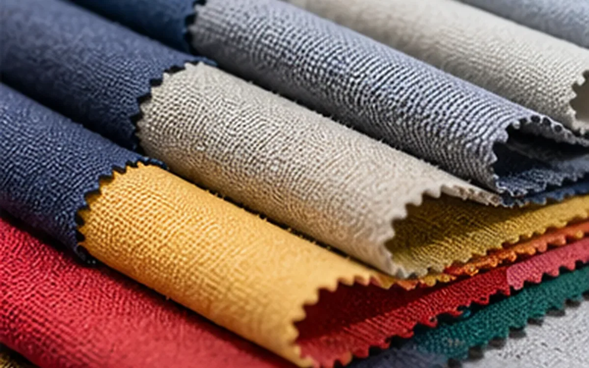
A fabric can contain more threads and still have the same calculated cover as another fabric. Finer yarns can offset the extra threads. Even when the cover values match, the gaps between yarns may have different sizes. A useful calculation must therefore say what it describes and what remains to be measured.
Woven cover factor helps compare yarn size with thread density. It can support fabric analysis and early design choices. It does not replace a test of airflow, strength, opacity or comfort. Nor does one number establish that a proposed construction can be woven on a particular loom.
The examples below are original teaching cases. Their construction values, yarn widths, image counts and airflow readings are invented. They show how to use the equations and check the units; they are not production results or recommended fabric specifications.
Name the kind of cover being reported
Several related quantities appear under the label cover factor. Before comparing two results, identify which one each report uses.
The conventional cotton cover factor combines threads per inch with yarn count in the English cotton system, Ne. It gives a useful construction index. A warp value of 16 on this scale is not a claim that warp covers 16% of the cloth.
Projected fractional cover describes the part of a flat view occupied by yarn. It runs from 0 to 1, or from 0% to 100% when expressed as a percentage. It can come from an ideal geometric model or from image analysis. Those two routes need not produce the same result on real cloth.
An open-area fraction is the complement of projected cover under the stated definition. It describes openings visible in that projection. It is not the same as the fraction of the fabric's three-dimensional volume occupied by voids. A yarn itself contains spaces between fibres, which a simple flat yarn-strip model does not describe.
CottonWorks identifies yarn size, thread count and weave design as influences on cover. That is a useful starting point. The calculation selected for a report must still state how it represents those features.
Get the construction inputs onto one basis
Ends per inch, or EPI, counts warp yarns across the fabric width. Picks per inch, or PPI, counts weft yarns along its length. These are thread densities, whereas Ne describes the yarn's length-to-mass relationship. Do not enter one kind of count in a field intended for the other.
Use the density measured in the fabric state being assessed. A loom setting, a relaxed grey sample and a finished roll can have different values. State whether the sample is relaxed, conditioned, stretched or taken at another defined stage.
ISO 7211-2:2024 covers the number of threads per unit length in woven fabrics. Its public scope describes three methods, with the choice depending on the fabric. The 2024 edition replaces the withdrawn 1984 edition. The laboratory needs the complete applicable method, including its counting and sampling rules.
Keep warp and weft inputs separate. A combined thread-count label does not tell you how those threads are divided between directions. It also tells you nothing about their yarn counts.
The cotton formula in this guide requires threads per inch. To convert threads per centimetre, multiply by 2.54. For example, 37.7953 ends/cm is approximately 96 EPI. Similarly, 28.3465 picks/cm is approximately 72 PPI. Use the unrounded measurements for the final calculation when available.
With 36 Ne warp yarn, entering 37.7953 directly in an EPI formula gives about 6.30. The correct factor for 96 EPI is 16. The wrong answer is smaller by a factor of 2.54 because the length unit was not converted.
Also check whether a yarn-count notation describes a single yarn or a folded assembly. The input must represent the actual yarn used in the cloth. Do not read the first number in a supplier's ply notation and assume it is the resultant count. ApparelDiary's yarn-count conversion guide explains the count systems used in these comparisons.
Calculate warp and weft factors before combining them
For the conventional cotton system, use:
Warp factor, Kw = EPI ÷ √warp Ne.
Weft factor, Kf = PPI ÷ √weft Ne.
Here, the square root applies to the yarn count alone. Use the whole count value, not a rounded square root taken from a chart.
Ömeroğlu, Akgun and Becerir's cotton-fabric research distinguishes the cotton-count convention from another expression using metric count. It also gives the combined Peirce expression:
Combined factor, Kc = Kw + Kf − (Kw × Kf ÷ 28).
The subtraction matters. Adding the two directional factors alone counts the projected overlap at warp–weft crossings twice.
For the starting example, suppose both yarn systems are 36 Ne. The fabric has 96 EPI and 72 PPI. Since √36 = 6:
Kw = 96 ÷ 6 = 16.
Kf = 72 ÷ 6 = 12.
Kc = 16 + 12 − (16 × 12 ÷ 28) = 21.1429, rounded.
The simple sum would be 28. It would miss an overlap correction of 6.8571. The corrected index is therefore about 21.14, not 28 and not 21.14%.
Keep the formula's convention visible. Replacing Ne with tex or Nm without changing the equation changes its meaning. A different counting system needs the correct conversion or its own stated expression. The number 28 belongs to this model and scale; it is not a universal constant for every fibre and yarn structure.
Read the combined factor through a geometric model
The meaning of the overlap term becomes clearer when each directional factor is divided by 28. Define the modelled warp fraction as a = Kw/28 and the weft fraction as b = Kf/28. Then:
Projected cover, C = a + b − ab.
Projected open fraction, O = (1 − a)(1 − b) = 1 − C.
This model treats the two yarn systems as regular, perpendicular strips in a flat view. Each system has a uniform width and spacing, with no overlap within that system. Real yarns can flatten, vary in width and move out of the assumed arrangement. The model's simplicity is useful, but it defines the limits of the result.
For the starting case, a = 16/28 and b = 12/28. The combined fraction is 21.1429/28 when rounded inputs are displayed. Using the exact values gives 75.51% projected cover and 24.49% projected open area.
The two directional covered fractions add to 100%. Yet the whole fabric is not fully covered in the model. Some warp-covered area lies over weft-covered area, while other parts remain open. This is why the combined value needs the overlap subtraction.
The result does not say that 24.49% of the fabric's volume is empty. It also does not say that 24.49% of incident light or a fixed fraction of airflow must pass through it. Those statements concern different measurements and mechanisms.
Calculate projected cover from stated yarn widths
A second route starts with thread density and the projected width of each yarn system. This avoids using yarn count as a proxy for width, though the width measurement itself still needs a clear method.
For a regular grid, multiply yarns per unit length by yarn width in the same length unit. The result is the directional covered fraction. A diameter measured from a free yarn may differ from its projected width after weaving, so identify which quantity was used.
Consider a separate invented fabric with these inputs:
Input | Warp | Weft |
|---|---|---|
Threads per centimetre | 32 | 24 |
Threads per millimetre | 3.2 | 2.4 |
Assumed projected yarn width, mm | 0.18 | 0.20 |
Directional covered fraction | 0.576 | 0.480 |
The warp fraction is 3.2 × 0.18 = 0.576. The weft fraction is 2.4 × 0.20 = 0.480. Combining them gives:
C = 0.576 + 0.480 − (0.576 × 0.480) = 0.77952.
The modelled cover is 77.952%, leaving 22.048% open area. The uncorrected sum would be 105.6%, another warning that directional cover cannot simply be added.
There is a second way to check the geometry. Warp spacing is 1/3.2 = 0.3125 mm. The clear gap is therefore 0.3125 − 0.18 = 0.1325 mm. Weft spacing is about 0.416667 mm, leaving a gap of about 0.216667 mm.
The rectangular opening has an area of about 0.0287083 mm². Its repeating cell occupies about 0.1302083 mm². Dividing opening area by cell area again gives 22.048%. The agreement checks the arithmetic within the assumed grid; it does not validate the assumed yarn widths against real fabric.
Equal cover can conceal different openings
Return to the cotton-count example and compare two constructions:
Construction | Warp and weft count, Ne | EPI | PPI | Kw and Kf | Modelled cover |
|---|---|---|---|---|---|
A | 36 | 96 | 72 | 16 and 12 | 75.51% |
B | 64 | 128 | 96 | 16 and 12 | 75.51% |
Construction B has more threads in both directions, but its yarns are finer. Since √64 = 8, its factors are 128/8 = 16 and 96/8 = 12. Both directional factors, and hence their combined cover, match construction A.
Within the ideal model, the thread spacings in B are three-quarters of those in A. To maintain the same directional fractions, the projected yarn widths also scale by three-quarters. Each clear-gap dimension then scales by the same amount.
The area of each opening becomes 0.75 × 0.75 = 0.5625 of the original. That is a 43.75% reduction in individual opening area, even though total open-area percentage stays the same. More, smaller openings occupy the same fraction of the surface.
This example does not predict which fabric will pass a filtration or airflow requirement. It shows why one total-cover value loses information about pore dimensions and distribution.
Kostajnšek and colleagues' optical study assessed pore number, size and distribution in transparent woven fabrics. Its work concerned plain and similar structures. Those are separate descriptions that a single average cover value cannot retain.
Test the effect of changing one construction input
Suppose construction A keeps its 96 EPI and 36 Ne yarns but increases weft density from 72 to 84 PPI. The warp factor remains 16, while the weft factor becomes 84/6 = 14.
New Kc = 16 + 14 − (16 × 14 ÷ 28) = 22.
The modelled cover becomes 78.57%, with 21.43% open area. Compared with the starting case, cover rises by about 3.06 percentage points. Open area falls by 12.5% relative to its original value.
Those percentages use different denominators. Neither is a measured reduction in air permeability. The calculation isolates the geometric change that follows from the stated inputs, provided the model remains suitable.
The proposed extra picks also need a production and product trial. Keep the other relevant yarn, weave and finishing conditions identified. If several inputs change, the resulting difference cannot be assigned to pick density alone.
Match the fabric state before comparing two reports
Thread density can change after the loom without adding a single yarn. If a fixed set of warp ends occupies less width, there are more ends per unit width. The same reasoning applies to picks when fabric length changes.
For a separate sensitivity case, let construction A's width fall to 95% of its starting width and its length to 97%. Assume the same ends and picks remain in the marked region. Finished densities become about 101.05 EPI and 74.23 PPI, respectively.
If yarn count is also held unchanged solely for this model, the recomputed projected cover is about 77.76%. It was 75.51% at the starting state. Comparing the two values as though they were measurements on identical fabric states would hide the dimensional change.
Real finishing can also alter yarn shape, mass basis and surface structure. The sensitivity case deliberately holds those features aside. It does not predict an actual finishing result or identify what caused the dimensions to change.
ApparelDiary's fabric shrinkage and pattern allowance guide covers the dimensional comparison in more depth. Keep the before-and-after measurements tied to the same defined treatment and sample basis.
Use images to measure the surface you actually have
Image analysis can estimate projected cover from a defined view of real cloth. It is especially helpful when a yarn-count model does not capture grouping, uneven spacing or the apparent width of yarns in the fabric.
Tàpias and colleagues used microscope images to measure woven-fabric cover. Their method included cropping to whole warp and weft periods, correcting uneven lighting and applying a threshold. The reported study used plain-weave sample groups; it does not validate every phone image or every fabric structure.
In a simple binary image, each accepted pixel is assigned either to an opening or to covered material. Suppose a valid analysis region contains 1,000,000 pixels and the chosen method identifies 250,000 as open. The projected open fraction is 25%, and cover is 75%.
Now change only the segmentation decision in this invented sensitivity check. If the open count becomes 240,000, cover becomes 76%. If it becomes 260,000, cover becomes 74%. That two-percentage-point spread comes from image classification, not a physical change in the cloth.
The example is not an uncertainty estimate for a camera or an instruction to tune the threshold until a desired result appears. Keep the raw image and the processing settings. Use a method suitable for the material, and check whether the result is stable under justified image-processing choices.
Lighting deserves particular care. Zupin and colleagues' 2024 study compared calculation and image analysis for 24 woven fabrics with different densities and weaves. Its abstract reports that illumination affected the results. The influence of threshold choice was smaller within that study's tested methods and fabrics.
Record the illumination, scale, focus, sample tension and region selected. Include enough of the repeat to answer the question. A crop chosen only because it looks clear may miss a grouped region or a sparse band.
Several images from one tiny area remain observations of that area. Samples taken from other positions or rolls provide different evidence. Report local values when the concern is uneven cover; a whole-roll mean can hide the weak region that prompted the investigation.
Average local cover after calculating it
Uneven fabric brings another calculation trap. The cover equation includes the product of two directional fractions, so applying it to average inputs need not give the average of the local cover values.
Consider two equal-area regions in an invented sample. Within each region, assume the regular-strip model is suitable. In region A, let a = 0.40 and b = 0.30. Its projected cover is 0.40 + 0.30 − 0.12 = 0.58, or 58%. In region B, let a = 0.80 and b = 0.70. Its cover is 0.80 + 0.70 − 0.56 = 0.94, or 94%.
Because the regions have equal areas, their average projected cover is (58% + 94%)/2 = 76%. That is the covered fraction for the whole two-region area under these assumptions.
Now average the directional fractions first. The average a is 0.60, and the average b is 0.50. Putting those values into the cover equation gives 0.60 + 0.50 − 0.30 = 0.80, or 80%. This is four percentage points higher.
The difference comes from the overlap. Its average local value is (0.12 + 0.56)/2 = 0.34. Multiplying the average fractions gives only 0.30, so too little overlap is subtracted.
When the question concerns overall projected area, calculate local cover and weight each result by the area it represents. Unequal regions need unequal weights. Keep the local results as well, since their variation may be the feature of interest. This example explains the averaging issue; it does not replace a laboratory method's sampling or reporting rules.
Measure airflow instead of converting cover into it
Air permeability depends on how air moves through the actual fabric. Pore shape, path length, yarn structure and deformation can matter alongside the visible openings.
Zhu and colleagues' cotton-fabric study considered yarn count, twist and packing density when predicting yarn diameter. Its public abstract also discusses pore geometry and pressure-dependent limits in airflow modelling. The study's fitted behaviour is not a general conversion from cover percentage to airflow.
ASTM D737-18(2023) covers air permeability of textile fabrics. Its public guidance explains that construction and finishing can change airflow paths. It also notes that the flow direction can matter when the two fabric surfaces differ.
ISO 9237:1995, confirmed in 2023, is another published air-permeability method. Select the method required for the product and follow its full procedure. Record the test pressure difference, test area, direction, sample state and reported units.
For a unit-conversion example only, assume a laboratory uses a 20 cm² area at a declared 100 Pa pressure difference. These are fictional case conditions, not instructions to select those settings for every fabric. Suppose the measured flow is 0.60 L/s.
Since 20 cm² equals 0.002 m², the area-normalised result is 0.60/0.002 = 300 L/(m²·s). This comes from a flow measurement. It cannot be obtained from the earlier 75.51% cover value.
Two results taken at different pressures or sample states should not be compared as though only construction had changed. The same caution applies to optical opacity, UV performance and comfort claims: specify and test the property needed for the intended use.
Recognise when the simple model has run out of room
The projected-grid equations require each directional covered fraction to lie between 0 and 1. If an assumed yarn width exceeds its pitch, the model has described overlapping strips within one yarn system. Its simple open-area calculation no longer represents that geometry.
For example, entering a = 1.10 and b = 0.50 gives C = 1.05 and O = −0.05. A fabric cannot have a negative projected open area. This is a model or input warning, not a physical result to report.
Check units, yarn width, fabric state and the arrangement of the yarns. Do not silently cap the answer at 100% and call it a measurement. A real construction can involve flattening, grouped yarns or different planes that the simple model omits.
Nor does a value below the model's limit prove that the cloth is easy to weave. Loom capability, interlacing and yarn behaviour still need assessment. Avoid universal labels such as good cover or maximum safe cover unless they belong to a clearly defined product and validated process.
Make the result useful in a fabric decision
A supplier comparison should retain the directional inputs, formula and fabric state beside the combined value. If the concern is visible gaps, add suitable images and local variation. If it is airflow, add the agreed permeability test. If it is cloth mass, measure mass per unit area rather than treating cover as a substitute.
ApparelDiary's fabric GSM testing guide explains that separate mass measurement. Fabrics can share a cover index while differing in yarn material, crimp, thickness or added finish. Those differences matter to the final product even when the cover calculation is correct.
Use cover to narrow a design question and explain a construction change. Preserve the original measurements so the next person can reproduce the calculation. The strongest report connects its cover value to a defined model and follows it with the evidence needed for the actual fabric decision.
References
CottonWorks: cover factor and the influence of yarn size, thread count and weave.
ISO 7211-2:2024: determination of the number of threads per unit length.
Tàpias and colleagues: Objective Measure of Woven Fabric's Cover Factor by Image Processing, 2010.
ISO 9237:1995: determination of the permeability of fabrics to air; confirmed in 2023.

Discussion0
Loading the discussion…