
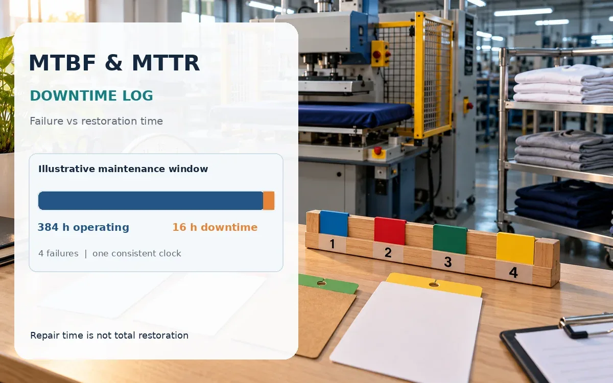
The maintenance report says average repair time is one hour, yet production lost sixteen hours across four breakdowns. Both figures can be correct if the first counts only hands-on work and the second includes response, diagnosis, parts waiting and checks. MTBF and MTTR calculation needs a defined event and a defined clock before it needs a formula. This guide reconciles one illustrative downtime log, separates repair from restoration and shows which result can support a factory availability discussion.
Define failure and restoration before collecting time
For a repairable machine, a functional failure is the loss of a stated required function. Define the function and the operating boundary: inability to run an approved cycle, loss of required output quality or another documented criterion. A minor adjustment, planned service and a production pause for missing material should not automatically become identical failure events in the maintenance metric.
Decide when the event starts. An alarm, operator recognition and actual loss of function may have different timestamps. Where the true start is unknown, state the recorded detection basis and uncertainty. Restoration ends when the machine has passed the agreed checks and is available for the required function, not when a technician leaves the work area or a work order is administratively closed.
MTTR can mean mean time to repair, restore or recover in different organisations. IBM's MTTR explanation includes the interval from failure to full functionality. Use an explicit label in your report, such as mean hands-on repair hours or mean failure-to-available hours. One abbreviation should not hide two different time boundaries.
Keep operating exposure separate from downtime
For the historical MTBF ratio, divide total relevant operating exposure by the count of functional failures within the defined scope. NIST's constant-rate reliability model uses total system operating time divided by total failures as the model's MTBF estimate. Record operating hours from a suitable counter or a reconciled state log; calendar hours since purchase are not the same exposure.
Decide how standby, idle but available time, reduced-speed running and planned stops are represented. The choice depends on the function and exposure model. Do not let each shift improvise a denominator. If a counter records motor-on hours but the failure mode depends mainly on cycles, retain cycle exposure as well and consider a cycle-based measure instead of assuming hours explain every failure mechanism.
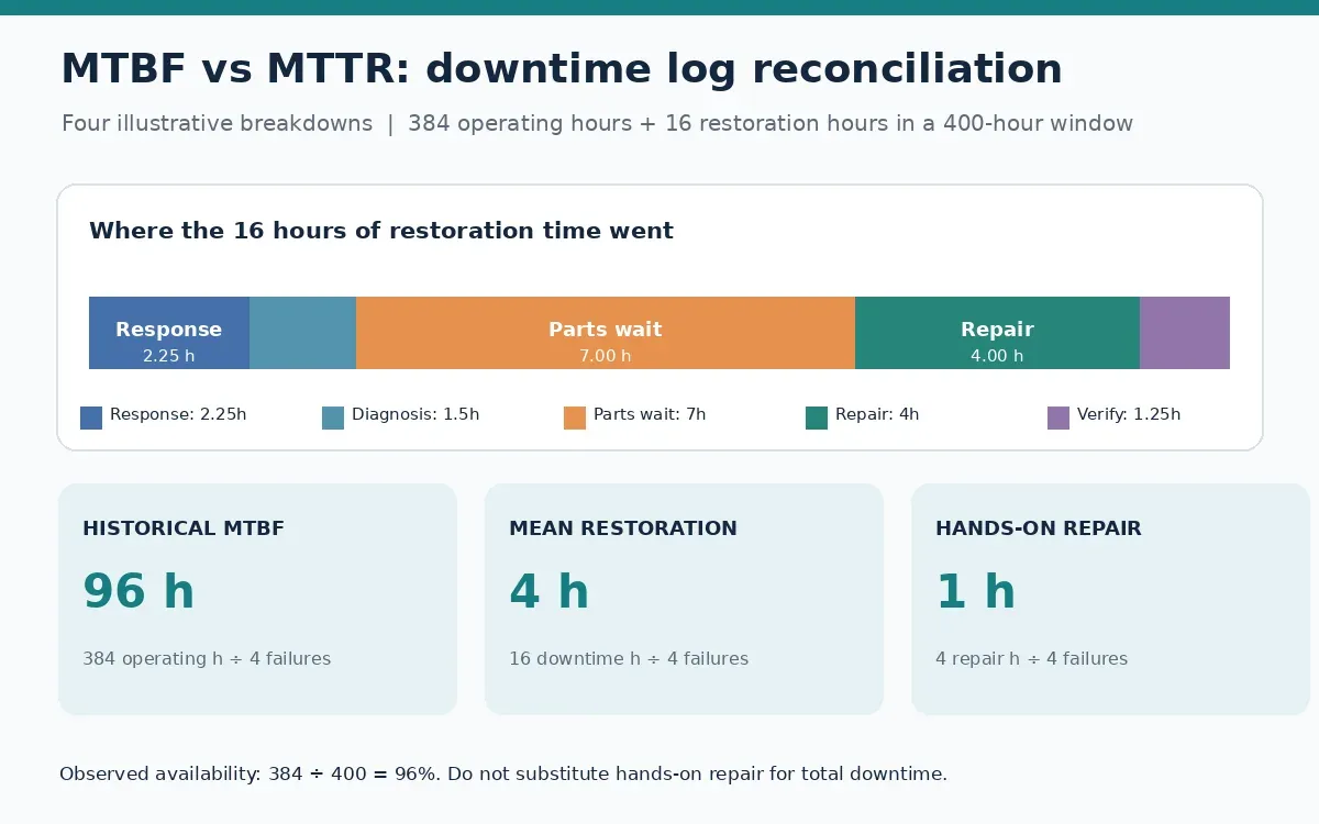
IBM's MTBF definition also notes that an average is not a promised life for a particular component. A recorded MTBF of 96 hours does not say the machine will fail at hour 96 or that preventive replacement should occur at that interval. Descriptive history and a validated reliability model are different levels of evidence.
Reconcile a four-event log
The following dataset is illustrative. One repairable asset has a 400-hour required window, consisting solely of 384 operating hours and 16 hours unavailable because of four functional failures. Each failure begins and is restored within the window. There are no other planned stops or loss categories in this simplified example. In a real report, those exclusions would need their own records.
All component times below are elapsed hours assigned to mutually exclusive stages on the restoration clock. They are not summed technician labour hours. If two technicians work together for one hour, the clock still advances one hour; labour effort is recorded separately.
Event | Response | Diagnosis | Parts wait | Repair | Verify | Total hours |
|---|---|---|---|---|---|---|
F1 | 0.50 | 0.50 | 2.00 | 1.00 | 0.25 | 4.25 |
F2 | 0.25 | 0.25 | 0.00 | 0.50 | 0.25 | 1.25 |
F3 | 1.00 | 0.50 | 4.00 | 1.50 | 0.50 | 7.50 |
F4 | 0.50 | 0.25 | 1.00 | 1.00 | 0.25 | 3.00 |
Total | 2.25 | 1.50 | 7.00 | 4.00 | 1.25 | 16.00 |
Historical MTBF is 384 divided by 4, or 96 operating hours per failure. Mean hands-on repair is 4 divided by 4, or 1 hour per repair. Mean failure-to-available restoration is 16 divided by 4, or 4 hours per event. The three figures answer different questions; retaining all three lets maintenance and production discuss the same log without forcing the clocks to agree artificially.
Parts waiting is 7 of the 16 restoration hours, or 43.75 percent. That is a useful investigation lead. It does not prove stocking every part will remove seven hours, because identification, approval, supplier availability and installation readiness may overlap or change. Trace the longest events to the relevant recovery path before approving a spares intervention.
Calculate availability only on a matching basis
For this simplified window, observed availability is operating time divided by operating plus failure downtime: 384 divided by 400, or 96 percent. The same result follows algebraically from 96 divided by the sum of 96 and 4, because the MTBF and mean restoration figures came from matching totals and the same event count.
Replacing restoration time with the one-hour hands-on repair value produces 96 divided by 97, or approximately 98.97 percent. That higher figure excludes twelve hours of response, diagnosis, parts waiting and verification from the denominator. It therefore does not describe the observed 400-hour window. Label any deliberately narrower metric by its actual scope rather than presenting it as production availability.
If your required window includes planned maintenance, material starvation, blocked output or idle-but-available states, define how each affects the metric. Actual runtime divided by all scheduled time and time available for operation divided by required time are not always the same quantity. A sewing-floor dashboard should also separate equipment availability from labour efficiency and quality; the site's factory KPI dashboard guide explains the importance of metric definitions.
Build a small data dictionary
One event identifier should link the operator loss record, maintenance work order, component issue and functional-release check. A follow-up task can share that identifier without being counted as another failure. Conversely, a confirmed new functional failure after restoration needs a distinct event, even if it has the same symptom as the previous one.
Field | Required definition | Typical owner |
|---|---|---|
Asset and function | Which item and approved function failed | Equipment owner |
Event start | Loss or detection basis with timestamp | Operator and supervisor |
Stage transitions | Response diagnosis wait repair and checks | Maintenance lead |
Available timestamp | Required checks passed and release recorded | Authorised release owner |
Exposure | Operating hours or cycles in the same scope | Counter or data owner |
Cause and action | Confirmed finding versus suspected mechanism | Engineer |
Keep unknown times marked as unknown. Do not fill a missing start timestamp with the work-order creation time merely to complete the table. If stage intervals overlap, either use a defined exclusive classification or report overlapping categories without adding them into a false total. The event's elapsed start-to-available interval should be reconciled independently.
Pool assets and periods with the right weights
When combining compatible assets or periods, add their operating exposure and failures, then calculate the ratio. Do not average the displayed MTBF values unless their weighting makes that arithmetic equivalent. The same principle applies to restoration: total matching elapsed restoration time divided by the matching restored-event count. A lightly used machine should not carry the same weight as one that contributed most of the exposure.
Keep incompatible populations separate. Different duty cycles, functions, product conditions or maintenance changes can make a plant-wide average unhelpful. Record deliberate changes and compare similar scopes. The site's preventive and predictive maintenance guide provides strategy context; the log here is the evidence needed to check whether a change affected failure occurrence, recovery or neither.
With zero failures, report zero observed failures and the exposure, with the simple MTBF ratio undefined. Do not publish zero MTBF or an infinite guaranteed life. NIST describes model-based bounds for zero-failure observations, but applying them requires the appropriate model, confidence convention and scope. A qualified analyst should review those assumptions before a management report claims a reliability lower bound.
Use the log to choose a focused intervention
A failure-rate problem and a long-restoration problem need different evidence. For repeated bearing damage, inspect the mechanical cause through the site's bearing failure guide rather than simply buying more replacements. For long parts waits, examine the approved spares path. For delayed functional checks, clarify release responsibility and access. None of those improvements requires weakening isolation or skipping a necessary verification.
Close each event with the required safe return-to-service checks, then retain the original timing record. Review a rolling period with its exposure and event count visible; a large swing based on one event deserves more caution than a stable pattern across many comparable events. Averages can conceal a long restoration tail, so retain individual durations and investigate outliers instead of reporting only the mean.
Start by reconciling one asset's next completed reporting window: required time, operating exposure, counted failures and total restoration hours. If those totals cannot agree, fix the state definitions before changing a target. Once they agree, the largest verified loss component gives maintenance a specific, measurable next task.


Discussion0
Loading the discussion…