
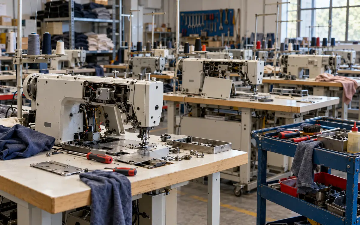
A maintenance team serves a fixed group of machines. When several machines stop at once, some wait for a technician. Their downtime grows beyond the time needed for the repair itself. The staffing question is therefore about both repair work and the queue before that work begins.
A finite source machine repair queue captures an important feedback effect. Only running machines can suffer a new operating failure in this model. As more machines stop, fewer remain able to join the repair queue. Treating failures as a fixed stream from an unlimited population can give a misleading answer.
This guide develops a complete example for eight fictional textile machines. It calculates the number waiting, mean downtime, machine availability and technician workload. It then compares one, two and three technicians using stated cost assumptions. Every numerical result comes from the model, rather than a claimed factory benchmark.
Recognize a finite source repair system
The machines circulate between two conditions: operating and down for repair. After repair, a machine returns to the operating group. It can then fail again after another operating period. The population stays fixed unless the planning scenario explicitly changes it.
This is the central idea in N. K. Jaiswal's finite-source queueing research. The same units return to the source population after service. A repair queue is one application of that structure.
Raj Jain's queueing-network notes explain the distinction between closed and open systems. They also discuss the machine repair model. The word closed concerns the circulating population. It does not mean that a factory has no material entering or leaving.
Imagine that all eight machines are running. All eight can generate a repair request. If five have stopped, only three running machines can produce the next request. A machine already waiting is not counted again as a fresh failure from the operating group.
This model concerns repair capacity. It differs from choosing the size of a physical buffer between production stages. ApparelDiary's factory buffer sizing guide covers that separate decision. It also differs from deciding which spare parts to stock, although missing parts may affect the repair process.
Define the assumptions before the formulas
Let N be the total number of machines and c the number of technicians. The machines are identical for this analysis. Each operating period is independent and has an exponential distribution with mean one divided by lambda. Each active repair is independent and exponential with mean one divided by mu.
Here lambda is the failure rate of one running machine. Its unit is failures per operating machine hour. Mu is the completion rate of one busy technician. Its unit is repairs per active repair hour. Neither is the observed total number of failures per calendar hour for the whole group.
One technician repairs one machine at a time. Waiting repairs begin as soon as a technician becomes free. The queue follows order of failure, and all technicians have the same repair rate. Travel, parts and restart work must either fit the defined service boundary or be modeled separately.
There are no shared failures, technician breaks, spare replacement machines or external repair jobs in the base case. Repaired machines return to the same operating-time model. The results describe long-run steady operation, rather than the first hour after a planned start with all machines healthy.
NIST's exponential distribution guide explains its constant hazard and reciprocal-mean properties. Constant hazard is an assumption to assess. It should not be imposed merely because a spreadsheet is easier to build with it.
If wear, aging, common utility faults or repair complexity drive the process, this simple model may be inadequate. Keep that limitation visible. A useful estimate depends more on a sound boundary and data than on the number of decimal places in the answer.
Describe the state and its changing rates
Let n be the number of down machines. This count includes machines waiting and machines under active repair. Its possible values run from zero through N. If n machines are down, N minus n remain operating.
The rate of the next failure therefore depends on n. The repair completion rate depends on how many technicians are busy. When there are fewer failed machines than technicians, some technicians are idle.
Failure rate in state n = (N − n) × lambda
Repair completion rate in state n = min(n,c) × mu
At n equal to zero, the repair completion rate is zero. At n equal to N, the failure rate is zero. Those boundaries are essential. They keep the state within the actual machine population.
János Sztrik's finite-source queueing notes present this classical birth-and-death model. A birth increases the number down by one. A death in the mathematical terminology is a repair completion that reduces that count by one.
No physical machine is destroyed by that label. It is simply a way to describe transitions between neighboring state counts. The distinction is useful when explaining the model to staff who use failure and repair language rather than queueing terms.
Calculate the long-run state probabilities
Write p(n) for the long-run probability of n machines being down. In steady state, the flow from n minus one to n balances the reverse flow. The failure rate in the first state times its probability equals the repair rate in the next state times its probability.
Instead of starting with unknown probabilities, begin with an unscaled weight w(0) equal to one. Generate each later weight from the preceding one. Divide all weights by their total at the end.
w(0) = 1
w(n) = w(n−1) × [(N−n+1) × lambda] ÷ [min(n,c) × mu]
Z = Sum of w(n), for n = 0 through N
p(n) = w(n) ÷ Z
The ratio has no unit because both rates use hours. The normalization step makes all probabilities add to one. This recurrence avoids manually expanding factorial formulas and is easy to audit row by row.
For a large population or extreme rate ratios, raw weights can overflow or become too small for software. A scaled recurrence or log calculation can help. Whatever method is used, check that probabilities are nonnegative, sum to one and satisfy the flow equations.
Work through eight machines and one technician
Assume each running machine operates for eight hours on average before failure. An active repair takes one hour on average. The base case has eight machines and one technician. These values are fictional teaching inputs, not recommended staffing targets.
N = 8; c = 1; lambda = 1 ÷ 8 = 0.125 per hour
mu = 1 ÷ 1 = 1 repair per hour
At state zero, failures occur at eight times zero point one two five, or one per hour. At state four, only four machines are running, so the failure rate is half a failure per hour. The technician still completes repairs at rate one while any failed machine is present.
The first weight is one times one divided by one, which equals one. The next is one times seven times zero point one two five, divided by one. It equals zero point eight seven five. Continuing the same calculation gives the following table.
Down machines n | Weight w(n) | Probability p(n), rounded |
0 | 1.000000 | 0.235570 |
1 | 1.000000 | 0.235570 |
2 | 0.875000 | 0.206124 |
3 | 0.656250 | 0.154593 |
4 | 0.410156 | 0.096621 |
5 | 0.205078 | 0.048310 |
6 | 0.076904 | 0.018116 |
7 | 0.019226 | 0.004529 |
8 | 0.002403 | 0.000566 |
The unrounded weights sum to about 4.245018. Dividing the first weight by that total gives p(0) of about 0.23557. Thus the technician has no repair demand for about 23.6 percent of time under these assumptions.
That idle share does not imply that waiting is negligible. Random failures can cluster, and a long repair can keep later failures waiting. The state distribution shows the full range from no failed machines to all eight down.
Convert the probabilities into useful measures
The expected number down, L, is the weighted sum of n. The expected number waiting, Lq, counts only the machines beyond the c active repair positions. The expected number operating is N minus L.
L = Sum of n × p(n)
Lq = Sum of max(n−c,0) × p(n)
Expected operating machines = N − L
For one technician, L is about 1.885 machines. Lq is about 1.120 machines. The expected operating count is about 6.115 out of eight.
These are averages over time, so they need not be whole numbers. They do not mean that part of a physical machine is waiting. A system that moves among integer states can have a fractional average.
The repair system's effective flow rate, X, follows from the machines that are actually running. Multiplying their average count by the per-machine failure rate gives the average number of failures per hour. In steady state, repairs must leave at the same rate.
X = lambda × (N − L)
X = 0.125 × (8 − 1.884562) = 0.764430 repairs per hour
As a separate check, the same rate equals mu times the expected number of busy technicians. For one technician, that busy count is one minus p(0). Both calculations give about 0.76443 repairs per hour.
The LINDO machine repair model also relates the operating population, total failure flow and downtime. Its example uses a different application. The same conservation idea still provides a check on the calculation.
Use the effective flow in Little's law
Mean downtime W includes both waiting and active repair. Mean queue wait Wq excludes active repair. Little's law links each mean time to the corresponding mean count using the flow that actually enters the repair system.
W = L ÷ X = 1.884562 ÷ 0.764430 ≈ 2.4653 hours
Wq = Lq ÷ X = 1.120132 ÷ 0.764430 ≈ 1.4653 hours
The difference is one hour, the mean active repair time. A repair that takes one hour of technician time therefore keeps a machine down for about two and a half hours on average in this case. Queue delay accounts for the extra time.
Using the all-machines-running rate of one failure per hour would understate both mean times. That rate applies only while all eight are running. It is not the long-run average flow through the repair queue.
NPTEL's explanation of Little's law emphasizes the rate of jobs actually entering the system. For this closed repair model, X supplies that rate. Using the correct population boundary is as important as using the formula correctly.
The average machine availability is the operating count divided by the total count. It is about 76.4 percent for one technician. This is availability within the stated repair model. It is not overall equipment effectiveness, output quality or a promise of shipped production.
Compare staffing alternatives on the same basis
Repeat the recurrence with two technicians and then three. Each technician still takes one hour per repair on average. The change is the number of repairs that can proceed at once. It is not a claim that two people halve the duration of one repair.
Measure | One technician | Two technicians | Three technicians |
Expected down machines | 1.8846 | 0.9942 | 0.8999 |
Expected waiting machines | 1.1201 | 0.1185 | 0.0124 |
Mean wait before repair, hours | 1.4653 | 0.1354 | 0.0140 |
Mean total downtime, hours | 2.4653 | 1.1354 | 1.0140 |
Machine availability | 76.44% | 87.57% | 88.75% |
Average utilization per technician | 76.44% | 43.79% | 29.58% |
Two technicians reduce average queue wait to about 8.1 minutes. Three reduce it further to less than one minute. The main improvement comes from the second technician; the third removes much less remaining waiting.
Average technician utilization falls as repair capacity increases. That can be the intended result when rapid response protects valuable equipment time. A policy that demands near-full technician utilization may create costly machine waiting.
Adding a second technician raises the effective flow from about 0.764 to 0.876 per hour. More machines are operating, so they generate more failures per calendar hour. The per-operating-hour failure tendency has not changed.
This distinction matters when reviewing a maintenance KPI. A larger repair count after a staffing improvement does not automatically show worse reliability. Compare operating exposure and failure rates, not just raw work-order totals.
Separate time-average congestion from arrival experience
With one technician, the technician is busy for about 76.4 percent of time. It is tempting to say that a new failure therefore waits with the same probability. That conclusion is wrong for this finite source model.
New failures occur more often in states with many machines still running. States with many failed machines generate fewer new arrivals. An arriving failure therefore sees a different state mix from an observer looking at a random time.
Weight each state probability by its failure rate to find the arrival view. Sum only states where all technicians are already busy, then divide by the total effective flow.
Probability a failure waits = [Sum for n ≥ c of (N−n) × lambda × p(n)] ÷ X
The result is about 69.2 percent for one technician. For two technicians it is about 19.8 percent. At a random time, both technicians are busy with probability of about 25.0 percent. That time-average measure answers a different question.
Neither probability is the chance that a repair lasts beyond a particular deadline. A target such as response within fifteen minutes needs a waiting-time distribution or a suitable simulation. Mean wait and probability of any wait answer narrower questions.
Price downtime and capacity transparently
For an illustrative comparison, assign a cost of thirty currency units per technician hour. Assign forty currency units per down machine hour. Assume the latter is a valid incremental loss for each affected machine and does not double-count technician cost.
Expected cost per hour = 30 × c + 40 × L
One technician costs about 105.38 units per hour. Two cost about 99.77. Three cost about one hundred and twenty-six. Two technicians have the lowest modeled cost among those choices.
The second technician reduces the expected down count by about 0.8903. At forty units per down machine hour, that benefit is about 35.61 units per hour. The added technician costs thirty, leaving a net modeled saving of about 5.61.
The break-even downtime value is 30 divided by 0.8903. It is about 33.70 units per machine hour. Above that value, the second technician is worthwhile under the stated inputs. Below it, the cost comparison favors one, unless a separate service constraint requires more capacity.
Do not use selling price per unit as downtime cost without checking the production system. A stopped machine may have spare capacity, a substitute route or work that can be recovered later. Conversely, a true bottleneck may affect an entire line. The simple additive loss model needs local evidence.
Build inputs from operating and repair records
Estimate failure rate from failure events divided by operating exposure. For example, record eighty failures across 640 operating machine hours. Dividing eighty by 640 gives the assumed rate of 0.125. Exclude time when a machine was already down from that operating exposure.
NIST's constant-rate estimation guidance uses total operating time and total failures. It also discusses uncertainty in the estimate. A point estimate from a small history should not be treated as an exact physical constant.
For the repair input, distinguish active repair service from queue delay. A recorded work-order duration may already include the wait for a technician. Do not use that whole duration as active service time. The queue model would then count the same waiting delay again. Define failure, service start, repair completion and return-to-operation timestamps clearly.
Classify parts delays and specialist waits. If a technician leaves a machine while waiting for a part, the machine is down but that technician may be free for other work. Treating the entire elapsed delay as continuous technician occupancy can overstate repair congestion.
ApparelDiary's critical spare parts guide addresses the stock decision behind some of those delays. Use the resulting service process in the repair queue. A technician count cannot stand in for a missing-parts policy.
Keep machine groups coherent. Compare failure rates, repair durations and skill needs across machines. Do not pool unlike groups into one average without testing the effect. A specialist may repair only some machines. The simple formula assumes all technicians can perform all modeled repairs.
Compare repair speed, reliability and staffing
Extra capacity is only one possible intervention. In the same eight-machine case, reduce mean active repair time from one hour to three quarters of an hour while keeping one technician. The calculated availability rises to about 84.2 percent.
Alternatively, keep the one-hour repair but increase mean operating time between failures from eight to ten hours. Availability becomes about 82.7 percent with one technician. These are separate changes, and neither includes the cost of achieving the improvement.
The comparisons show where a more detailed business case is needed. Better diagnosis, prepared tools or parts access may shorten service. A reliability project may reduce failures. Another technician may reduce queue delay. Each changes a different part of the model and needs its own evidence.
Even with a technician available for every machine, repairs still take time. Under the base inputs, removing all queue wait gives availability of eight divided by nine. That is about 88.9 percent. More repair capacity cannot remove the one-hour service time itself.
Make a spreadsheet that exposes its own checks
Use one row for every possible down count, including zero and all N machines. Place the operating count, failure rate and repair rate beside that state. The first row has no repair completion. The final row has no further operating failure. Those two boundary rows catch many indexing mistakes.
In the weight column, each row uses the previous row's failure rate and the current row's repair rate. Using both rates from the current row is a different recurrence and gives the wrong distribution. Keep the formula references visible rather than replacing them with pasted values.
After normalization, multiply each down count by its probability. Do the same for each waiting count in another column. Their sums produce L and Lq. Use another column for busy technicians times probability. This gives the service-side flow check. It should agree with the flow calculated from operating machines.
Check the inputs before calculating. The population and technician count must be positive whole numbers for this model. Mean operating and repair times must be positive and use the same time unit. A missing repair mean must not become zero through a default cell value.
The worked results were checked with a second calculation. It solves the full stationary balance equations independently. Agreement between two methods helps detect a formula error. It does not validate the assumed failure pattern or the quality of the maintenance records.
Retain full precision in the calculation and round only the displayed results. Rounded state probabilities may not sum exactly to one. Do not adjust a convenient row by hand to hide that display effect, because it would alter the model's evidence trail.
Save the input version, date and staffing scenario with each output. A result without those details is hard to reproduce during a later review.
Match the time horizon to the decision
A steady-state average describes a system observed over a long enough period under stable rules. It does not predict the exact queue at the next shift start. If all machines start healthy, the early state mix differs from the long-run mix. If several machines arrive at the shift already down, the initial repair burden is larger.
Record that initial condition when judging a short staffing change. A relief technician for the first hour may serve an inherited backlog. A technician available throughout a long campaign serves repeated failures as well. Those two duties should not be compared by assigning the same long-run average benefit to every paid hour.
The operating clock also needs a clear definition. If machines stop during an unstaffed period, their operating-failure exposure pauses under this model. Repairs may pause too. If production continues overnight while repair staff leave, the queue follows a different calendar and can build until service resumes.
Do not multiply an hourly steady-state saving by all calendar hours without checking those conditions. Use the actual operating and repair windows for the business case. When the windows differ materially, a transient calculation or simulation can represent the starting backlog and the changing capacity. Preserve the simple steady-state case as a benchmark for checking the richer model.
Move to simulation when the operating rules matter
A shift with meal breaks and an overnight repair backlog does not resemble constant steady staffing. Common failures can stop several machines together. Some repairs require two people, and others wait for a specialist or a test fixture. These rules may require a richer model.
SimPy's machine shop example demonstrates machines that fail and compete for a repair resource. It also includes other work that can be interrupted by repairs. Its repair-time assumptions differ from this exponential example. Match those inputs before using its results as a direct check.
When building a simulation, first reproduce a simple case whose analytical answer is known. Then add the real calendars, skills, delays and distributions one at a time. Use repeated runs and appropriate uncertainty analysis before comparing staffing alternatives.
Frequently asked questions
Why not use an ordinary M/M/1 queue?
That model assumes a fixed external arrival rate. Here, new repair demand declines as the operating population shrinks. Using the initial rate of one per hour with a service rate of one gives no stationary open-queue result. The finite source model still has a valid bounded state distribution.
Does a bounded queue mean staffing is adequate?
No. At most eight machines can be down because only eight exist. A bounded queue can still imply poor availability and long waits. Judge staffing against service needs and credible costs, not just mathematical stability.
Can two technicians work together on one repair?
The base model assumes parallel independent repairs, one person per machine. A joint repair has a different resource requirement and may have a different duration. Model that work explicitly rather than multiplying the service rate without evidence.
Make the staffing decision traceable
The finite source repair model links technician capacity to the number of machines that remain able to fail. In the worked case, a second technician sharply reduces waiting and has the lowest stated hourly cost. The result depends on the repair boundary, rates and downtime value.
Keep those assumptions beside the recommendation. Recalculate when the machine population, staffing calendar or failure pattern changes. The model then provides a way to compare repair capacity choices. It also explains how lower technician utilization can support better machine availability.
Repair staffing links to reliability data, so see MTBF and MTTR calculation, preventive versus predictive maintenance and queuing theory.
References
1. N. K. Jaiswal: Finite-Source Queuing Models. Finite populations whose members return after service.
2. Raj Jain: Queueing Networks. Closed networks and the machine repair model.
3. János Sztrik: Finite-Source Queueing Systems and Their Applications. Classical repair model, state-dependent rates and arrival observations.
4. NIST: Exponential Distribution in Reliability. Constant hazard and mean operating time.
5. LINDO: Machine Repair Model EZMREPAR. Operating population, effective flow and downtime relationships.
6. NPTEL: Little's Result. Counts, actual arrival rates and mean times.
7. NIST: Constant Repair Rate Model Estimation. Failure-rate and MTBF estimation from operating exposure.
8. SimPy: Machine Shop. Simulation of machine failures, repair resources and other work.


Discussion0
Loading the discussion…